CMOS Logic Gates: Inverter, NAND, and NOR


CMOS Logic Gates: Inverter, NAND, and NOR

Complementary metal–oxide–semiconductor (CMOS) technology forms the backbone of modern digital IC design. Patented by Frank Wanlass in 1963 (US patent 3,356,858), CMOS enables low-power, high-speed, and noise-immune logic circuits. CMOS gates, including inverters, NAND, and NOR, are widely used in both large-scale and small-scale integrated circuits due to their efficiency and versatility.

CMOS Inverter

A CMOS inverter consists of a complementary pair of PMOS and NMOS transistors. The PMOS transistor connects to the supply voltage VDD, while the NMOS connects to ground. The input voltage VIN controls both gates, and the output voltage VOUT is taken from the connected drains. CMOS inverters are highly energy-efficient and produce minimal heat due to their complementary switching.
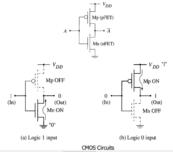
Working principle of CMOS inverter showing PMOS and NMOS operation
Fig.1. Working of CMOS Inverter

DC Analysis of CMOS Inverter

DC analysis determines the voltage and current characteristics of the inverter under steady-state conditions. This helps ensure that each transistor operates within safe limits and identifies the node voltages, mesh currents, and branch voltages.
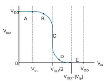
Operating regions of CMOS inverter showing transistor states
Fig.2. Operating regions of CMOS Inverter

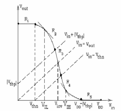
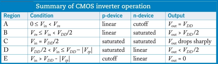
The CMOS inverter’s operation can be divided into five regions:

  • Region A: NMOS cutoff, PMOS linear, output ≈ VDD
  • Region B: NMOS saturation, output starts decreasing
  • Region C: Both transistors saturated, sharp drop in output
  • Region D: NMOS linear, PMOS saturation
  • Region E: PMOS cutoff, output ≈ 0
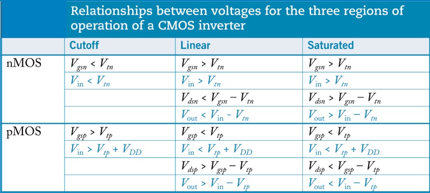
Table showing relationship between CMOS inverter operating regions
Table 1. Relationship between Operating regions of CMOS Inverter
Voltage transfer characteristic curve of CMOS inverter
Fig.3. Voltage Transfer Characteristic (VTC) of CMOS Inverter

Noise Margin

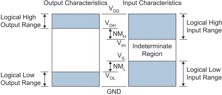
Noise margin quantifies the tolerance of a CMOS gate to input noise without affecting the output. It includes:

  • NL = VIL – VOL
  • NH = VOH – VIH
Noise margin definitions showing VIH, VIL, VOH, VOL
Fig.4. Noise Margin Definitions

Transient Analysis

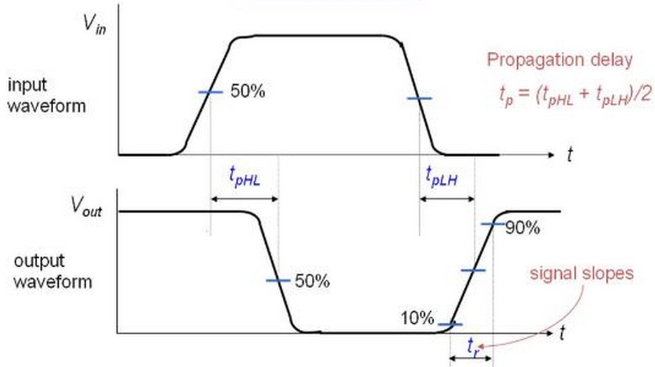
Transient analysis examines the time-dependent response of CMOS gates, measuring rise/fall times, propagation delays, and switching behavior. This analysis helps evaluate the performance of gates under dynamic conditions.
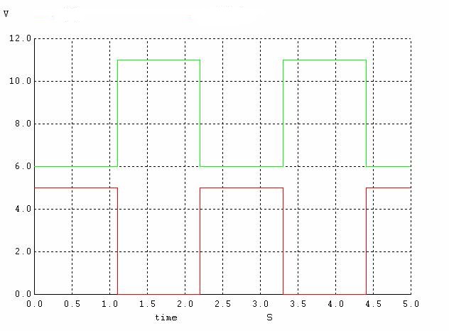
Transient response waveform of CMOS inverter
Fig.5. Transient Response of CMOS Inverter

The rise and fall times depend on the "on" resistance of transistors and load capacitance, including input capacitance, interconnect wiring, and board capacitance.
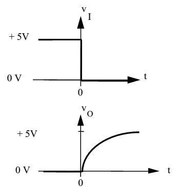
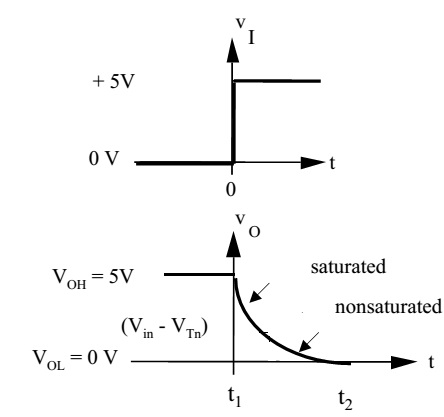
Rise time low to high transition waveform
Rise time: Low-to-High Transition
Fall time high to low transition waveform
Fall time: High-to-Low Transition
Propagation delay waveform of CMOS inverter
Fig.6. Propagation Delay of CMOS Inverter
Summary table of CMOS inverter operation
Table 2. Summary of CMOS Inverter Operation

CMOS NAND & NOR Gates

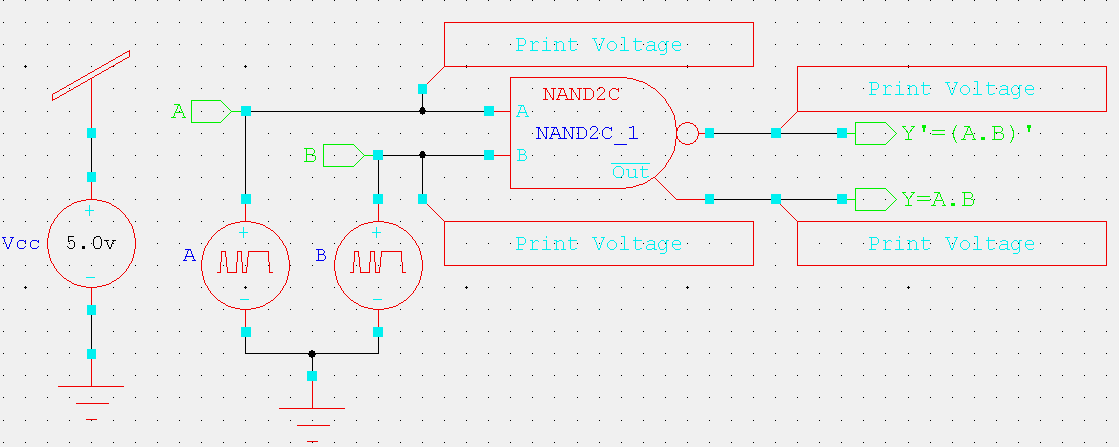
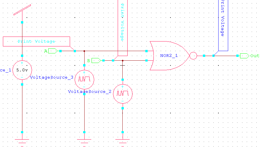
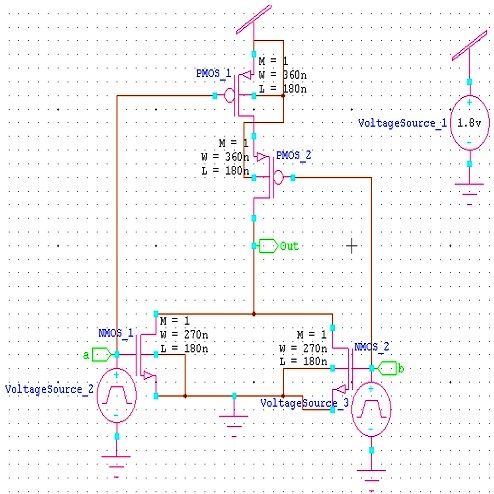
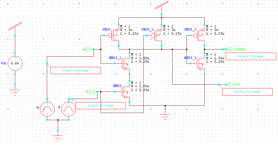
NAND and NOR gates are fundamental building blocks of digital logic. CMOS implementations provide low power, high density, and fast switching. The layout of these gates differs in transistor configuration:

  • NAND: PMOS in parallel, NMOS in series
  • NOR: PMOS in series, NMOS in parallel
CMOS NAND gate schematic
Fig.9. CMOS NAND Gate
Transient response of CMOS NAND gate
Fig.10. Transient Response of NAND Gate
CMOS NOR gate schematic
Fig.11. CMOS NOR Gate
Transient response of CMOS NOR gate
Fig.12. Transient Response of NOR Gate

SPICE Simulation and Waveforms

T-Edit allows extraction of SPICE code from schematics for simulation. W-Edit provides waveform visualization, enabling designers to verify input-output behavior and transient response accurately.

Conclusion

CMOS inverters, NAND, and NOR gates demonstrate efficient low-power logic operation with predictable DC and transient characteristics. Tanner EDA tools streamline design, simulation, and waveform analysis, ensuring reliable digital IC development.

l

Further Reading

  1. Introduction to Tanner EDA Tools
  2. EDA Tools and VHDL for VLSI Design
  3. Layout of CMOS Inverter
  4. Standard Cell Design in VLSI
  5. Design of CMOS XOR/XNOR Gates
  6. Design of CMOS Full Adder
  7. Design of CMOS Flip-Flops (SR, D, JK)
  8. Design of 8-bit Synchronous Counter
  9. Design of 8-bit Bi-Directional Register
  10. Design of a 12-bit CPU with Basic Instructions
  11. VHDL Logical Function & CMOS Inverter
  12. CMOS Layout Color Codes - IC Design Guide


Contact Us

Name

Email *

Message *

Popular Posts

Q-function in BER vs SNR Calculation (with Simulation)

Q-function in BER vs. SNR Calculation In digital communications and signal processing, the Q-function plays a significant role in predicting system reliability. It allows engineers to quantify the probability that Gaussian noise will exceed a specific threshold, causing a bit error. What is the Q-function? The Q-function is a mathematical function representing the tail probability of the standard normal (Gaussian) distribution. It is the complementary cumulative distribution function (CCDF) of a standard Gaussian distribution. Q(x) = (1 / √(2Ï€)) ∫â‚“∞ e^(-t² / 2) dt Q-Function Interactive Simulator Move the slider to see how the "Tail Probability" (the area in red) changes. This area represents the Probability of Error (BER) . Threshold Distance ( x ) — (Simulates Increasing SNR) x = 1.0 Q(x) = 0.1587 ...

BER vs SNR for M-ary QAM, M-ary PSK, QPSK, BPSK, ...(MATLAB Code + Simulator)

Bit Error Rate (BER) & SNR Guide Analyze communication system performance with our interactive simulators and MATLAB tools. 📘 Theory 🧮 Simulators 💻 MATLAB Code 📚 Resources BER Definition SNR Formula BER Calculator MATLAB Comparison 📂 Explore M-ary QAM, PSK, and QPSK Topics ▼ 🧮 Constellation Simulator: M-ary QAM 🧮 Constellation Simulator: M-ary PSK 🧮 BER calculation for ASK, FSK, and PSK 🧮 Approaches to BER vs SNR What is Bit Error Rate (BER)? The BER indicates how many corrupted bits are received compared to the total number of bits sent. It is the primary figure of merit f...

Pulse Width Modulation (PWM)

Pulse-width modulation (PWM), or pulse-duration modulation (PDM), is a method of controlling the average power delivered by an electrical signal.   Fig: An example of PWM in an idealized inductor driven by a blue line voltage source modulated as a series of sawtooth pulses, resulting in a red line current in the inductor.    Generating a PWM Signal The simplest way to generate a PWM signal is the intersection method, which requires only a sawtooth or a triangle waveform (easily generated using a simple oscillator) and a comparator. When the value of the reference signal is more than the modulation waveform, the PWM signal (magenta) is in the high state; otherwise, it is in the low state.      Duty cycle A low duty cycle equates to low power because the power is off for most of the time; the word duty cycle reflects the ratio of "on" time to the regular interval or "period" of time. The duty cycle is measured in percent, with 100% representing full o...

Frequency Shift Keying (FSK) Modulation & Demodulation (with Simulation)

Frequency Shift Keying (FSK) Theoretical Foundations: Frequency Shift Keying (FSK) is a discrete frequency modulation scheme wherein the digital information is encoded via instantaneous shifts in the carrier signal's frequency. The fundamental implementation is Binary FSK (BFSK), which maps binary data onto two distinct, discrete spectral states. A binary '1' (the "mark" state) is represented by a carrier frequency \( f_1 \), while a binary '0' (the "space" state) corresponds to frequency \( f_2 \). Each symbol is sustained for a bit interval denoted by \( T_b \). FSK Transmitter Characterization: The mathematical model for the modulated BFSK output \( s(t) \) is defined as: \[ s(t) = \begin{cases} A_c \cos(2\pi f_1 t), & \text{for } m = 1 \\ A_c \cos(2\pi f_2 t), & \text{for } m = 0 \end{cases} \] ...

FFT Butterfly Method Explained (with Example of 4-point DFT)

  FFT Using Butterfly Method Given: x[n] = {0, 1, 2, 3} Step 1: Split into Even & Odd Even indices: x e = {0, 2} Odd indices: x o = {1, 3} Step 2: 2-point DFT For any {a, b}: DFT = {a + b, a - b} Even Part: E = {0+2, 0-2} = {2, -2} Odd Part: O = {1+3, 1-3} = {4, -2} Step 3: Combine Using Butterfly X[k] = E[k] + W k O[k] X[k + N/2] = E[k] - W k O[k] For N = 4: W 0 = 1 W 1 = -j Final Calculations X[0] = 2 + 4 = 6 X[2] = 2 - 4 = -2 X[1] = -2 + (-j)(-2) = -2 + 2j X[3] = -2 - (-j)(-2) = -2 - 2j Final Answer: X[k] = {6, -2 + 2j, -2, -2 - 2j} Try Interactive Online Simulations Interactive FFT Online Simulator (For understanding Fundamentals)  Interactive FFT Online Simulator (Analyze .CSV, .MP3, .MP4, etc. Further Reading Fourier Transform OFDM Return to Fourier Transform Main Page →

Design of CMOS Flip-Flops (SR, D, JK)

Design of CMOS Flip-Flops (SR, D, JK) A flip-flop or latch is a circuit with two stable states, used to store state information. It is the basic storage element in sequential logic and a fundamental building block in digital electronics systems, including computers and communication devices. Flip-flops and latches act as data storage elements for states, pulse counting, and synchronization of variably-timed input signals to a reference clock. Flip-flops can be transparent/opaque (latches) or clocked (synchronous, edge-triggered). Latches are level-sensitive, while flip-flops are edge-sensitive. In sequential logic, the output depends on current inputs and previous states. Fig.1 shows a sequential circuit combining a combinational block and a memory element. ...

AM Modulation Online Simulator

Amplitude Modulation Simulator s AM (t) = A c [1 + k a m(t)] cos(ω c t) where, ω = 2πf & k a = Amplitude Sensitivity Modulation index, μ = k a A m Message Frequency (fm): Carrier Frequency (fc): Carrier Amplitude (Ac): Modulation Index (m = Am / Ac):