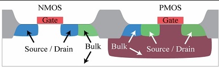
Layout of CMOS Inverter


Layout of CMOS Inverter

Layout is the process of drawing different mask layers of an IC. Each layer is drawn using a specific color and follows a set of design rules that act as an interface between the designer and the process engineer. Typical considerations include spacing, minimum width, overlap, manufacturability, performance, IC size, and parasitic elements.
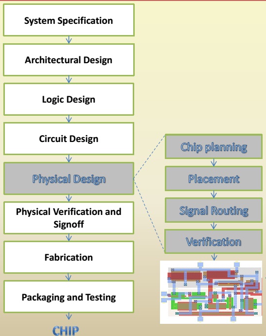
Layout design flow in VLSI
Fig.1. Layout Flow

Design Rules

Design rules are categorized as Lambda (位) rules and Micron rules:

1. Lambda-based rules

  • Scalable rules based on a constant parameter (位).
  • 2位 equals minimum channel length; allows process portability.
  • Processes rarely shrink uniformly, so adjustments may be needed.

2. Micron-based rules

  • Minimum sizes and spacing specified directly in microns.
  • Not tied to 位 multiples; can reduce area by ~50% compared to 位 rules.

Types of design rules include:

  • Intra-layer: Width, spacing
  • Inter-layer: Enclosures, distances, overlaps
  • Specific rules: Antenna, density, minimum area
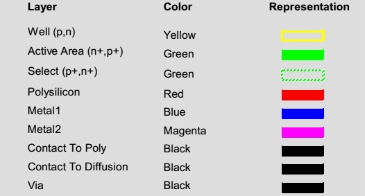
CMOS fabrication process layers
Fig.2. CMOS Process Layers
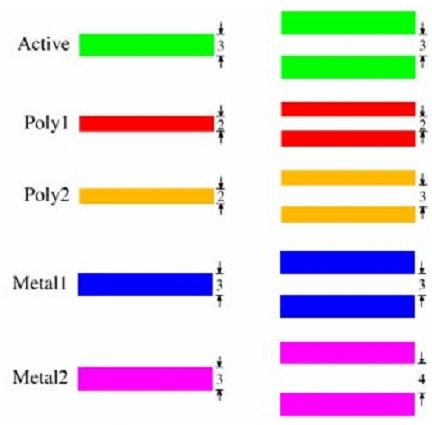
Intra layer design rules illustration
Fig.3. Intra Layer Design Rules

The 位 rules were introduced by Mead and Conway (1980) to allow scalable, portable designs. The MOSIS service provides standard 位-rule sets for academic and commercial designs.
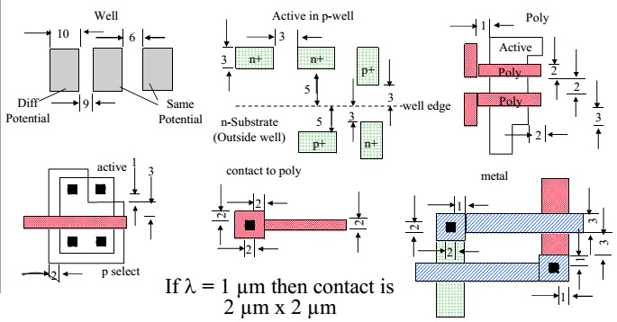
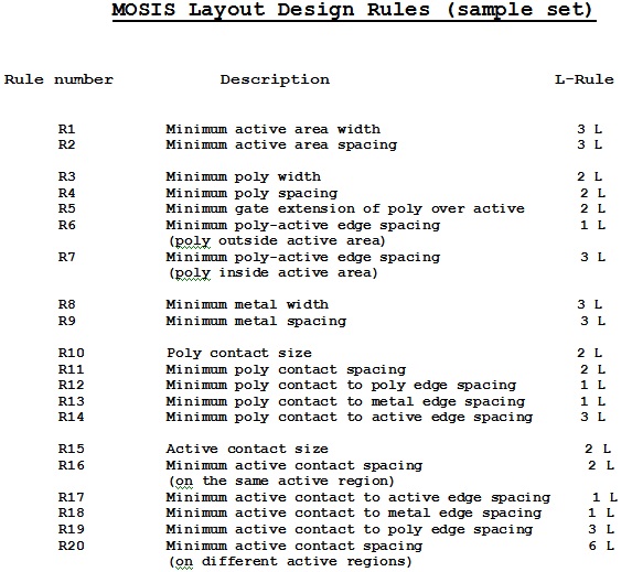
MOSIS lambda based design rules
Fig.4. MOSIS 位-Based Design Rules
Lambda based design rules diagram
Fig.5. Lambda-Based Design Rules

CMOS Inverter Layout

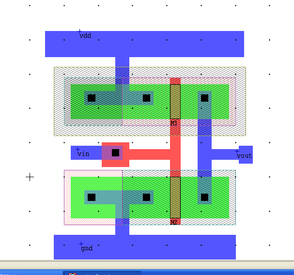
Layout of CMOS inverter in L-Edit
Fig.6. Layout of CMOS Inverter

The layout is drawn in L-Edit following 位 rules and CMOS process layers. After layout generation, it must pass:

  • Design Rule Check (DRC): Automatically verifies that layout polygons follow all design rules.
  • Layout versus Schematic (LVS) check: Ensures the layout matches the original circuit schematic.
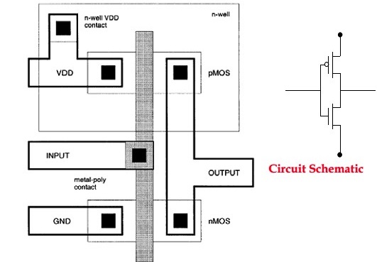
Structure of CMOS inverter layout
Fig.7. Structure of the Layout of CMOS Inverter

Cross-Sectional View

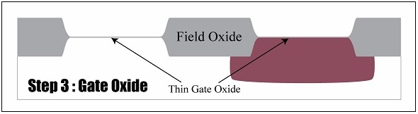
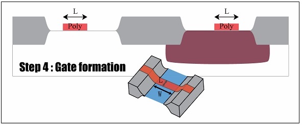
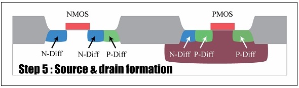
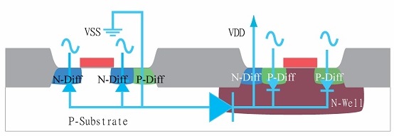
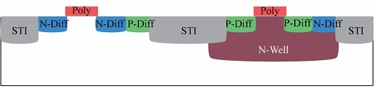
L-Edit allows visualizing the cross-section of the CMOS device, showing the fabrication steps. Observe the drains, sources, gates, and bulks of NMOS and PMOS transistors:
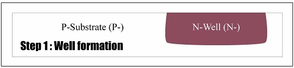
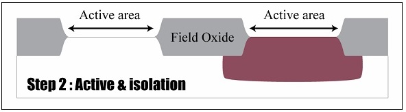
Cross section view step 1 Cross section view step 2 Cross section view step 3 Cross section view step 4 Cross section view step 5 Cross section view step 6 Cross section view step 7 Cross section view step 8

Key observations:

  • Drain and Source are fabricated similarly.
  • All NMOS bulks are connected together.
  • All PMOS bulks in the same N-well are connected together.

SPICE Programming and Graphs

SPICE code can be extracted using T-Edit, and simulations with W-Edit produce the corresponding graphs for verification.

Conclusion

The CMOS Inverter layout drawn using L-Edit was successfully verified using DRC, LVS, and SPICE simulations. The process demonstrated proper adherence to design rules and layout correctness.


Further Reading

  1. Introduction to Tanner EDA Tools
  2. CMOS Logic Gates: Inverter, NAND, and NOR
  3. EDA Tools and VHDL for VLSI Design
  4. Standard Cell Design in VLSI
  5. Design of CMOS XOR/XNOR Gates
  6. Design of CMOS Full Adder
  7. Design of CMOS Flip-Flops (SR, D, JK)
  8. Design of 8-bit Synchronous Counter
  9. Design of 8-bit Bi-Directional Register
  10. Design of a 12-bit CPU with Basic Instructions
  11. VHDL Logical Function & CMOS Inverter
  12. CMOS Layout Color Codes - IC Design Guide


Contact Us

Name

Email *

Message *

Popular Posts

Hybrid Beamforming | Page 1

Beamforming Techniques Hybrid Beamforming... Page 1 | Page 2 | Hybrid Beamforming: Hybrid beam formation was developed to address some of the limitations of digital pre-coding approaches. Every antenna element is connected to an RF chain in digital pre-coding (beam forming) method. We also know that each RF chain is in charge of providing a separate data stream between the transmitter and the receiver. We know that a larger number of independent data streams leads to higher data rates. It has a spatial multiplexing feature for MIMO. As a result, we may assume that switching from MIMO to massive MIMO will benefit us more in terms of spatial multiplexing in massive MIMO, where each antenna is coupled to a single RF chain. We'll proceed with a definition of hybrid beam forming. Overview of hybrid beam forming with example: Unlike digital beam forming, more than one antenna element is connected to a single RF chain in hybr...

UGC NET Electronic Science Previous Year Question Papers with Solutions

Home / Engineering & Other Exams / UGC NET 2026 PYQ ⬇️ Download Papers and Solutions 馃搵 Exam Pattern 馃挕 Preparation Tips ❓ FAQs 馃搳 Exam Highlights: Electronic Science (88) Feature Details Junior Research Fellowship (JRF) ₹37,000 + HRA per month Eligibility M.Sc/M.Tech in Electronics (55%) Validity of Certificate JRF (3 Years) | Lectureship (Lifetime) 馃摜 Download UGC NET Electronics PDFs Complete collection of previous year question papers, answer keys and explanations for Subject Code 88. Start Downloading 馃搨 View All Question Papers June 2025 - Question Paper Download PDF June 2025 - Solved Paper + Explanation ...

MATLAB Code for 8-PSK, 16-PSK, ...

馃摌 Overview & Theory 馃М MATLAB Code for BPSK, QPSK, 8-PSK, 16-PSK, 32-PSK 馃М Simulator for m-ary PSK 馃摎 Further Reading   MATLAB Code for BPSK, QPSK, 8-PSK, 16-PSK, 32-PSK clc; clear all; close all; rng(10) M = 8; % M = 2, 4, 8, 16, 32, etc. N_Bits = 2520; Phase = 0; data_info_bit = randi([0,1],N_Bits,1); data_temp = bi2de(reshape(data_info_bit,N_Bits/log2(M),log2(M))); modData = pskmod(data_temp,M,Phase); figure(1); scatterplot(modData); channelAWGN = 15; rxData2 = awgn(modData, channelAWGN); figure(2); scatterplot(rxData2); demodData = pskdemod(rxData2,M,Phase);   for BPSK, Constellation Size, M = 2 for QPSK, M = 4 for 8-PSK, M = 8, and so on    Output Figure: 8-PSK Modulation Figure: 8-PSK Demodulation after adding AWGN Noise Using the above MATLAB code you'll able be to modulate and demodulate 2-PSK, 4-PSK, 8-PSK, 16-PSK, 32-PSK and so on.  16-PSK   Fig: 16-PSK In this above code ' M ' is the number of the conste...

MIMO Channel Matrix | Rank and Condition Number

MIMO / Massive MIMO MIMO Channel Matrix | Rank and Condition...   The channel matrix in wireless communication is a matrix that describes the impact of the channel on the transmitted signal. The channel matrix can be used to model the effects of the atmospheric or underwater environment on the signal, such as the absorption, reflection or scattering of the signal by surrounding objects. When addressing multi-antenna communication, the term "channel matrix" is used. Let's assume that only one TX and one RX are in communication and there's no surrounding object. Here, in our case, we can apply the proper threshold condition to a received signal and get the original transmitted signal at the RX side. However, in real-world situations, we see signal path blockage, reflections, etc.,  (NLOS paths [↗]) more frequently. The obstruction is typically caused by building walls, etc. Multi-antenna communication was introduced to address this issue. It makes diversity app...

OFDM Symbols and Subcarriers Explained

This article explains how OFDM (Orthogonal Frequency Division Multiplexing) symbols and subcarriers work. It covers modulation, mapping symbols to subcarriers, subcarrier frequency spacing, IFFT synthesis, cyclic prefix, and transmission. Step 1: Modulation First, modulate the input bitstream. For example, with 16-QAM , each group of 4 bits maps to one QAM symbol. Suppose we generate a sequence of QAM symbols: s0, s1, s2, s3, s4, s5, …, s63 Step 2: Mapping Symbols to Subcarriers Assume N sub = 8 subcarriers. Each OFDM symbol in the frequency domain contains 8 QAM symbols (one per subcarrier): Mapping (example) OFDM symbol 1 → s0, s1, s2, s3, s4, s5, s6, s7 OFDM symbol 2 → s8, s9, s10, s11, s12, s13, s14, s15 … OFDM sym...