Digital Beamforming for Multi-User scenario

Baseband precoding:

Baseband precoding is to cancel interferences between multi stream in MIMO communication. Here in hybrid precoding each RF chains are connected to more than one antenna element. And each RF chain responsible of one data stream

The signal that has been sent can be denoted as.

x=Ds........................................................(i)

Where, x = transmitted signal vector

D = N_t X N_r digital precoder

s = N_r X 1 symbol vector

Now, received signal vector y at receiver side,

y= √ρHDs + n…………………………….. (ii)

Here, ρ = average received power

H =channel matrix ( N_r X N_t)

n = additive white Gaussian noise vector

Digital Beamforming for Multi-User scenario

Here in above figure 6.2, BS uses N_BS antennas and N_BS^RF chains for communication with U mobile stations (MSs) simultaneously. N_MS antennas are there in each MS. The total number of data streams for communication is equal to the number of antennas on the receiver side, N_MSU, where N_MSU ≤ N_BS. On the downlink side, the BS applies an N_BS X N_MSU digital precoder D

Where, D= [D₁, D₂, …, D_U],

D_u = For the u th user, a digital precoder (size of N_BS X N_MS)

At the u th MS, the received signal vector r_u is now denoted by, …………………………………………………………....(iii)

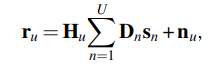
Where, s_n = original signal vector of size N_MS X 1

H_u = represents channel matrix between the base station and the u^th MS

n_u =AWGN vector with zero mean and standard deviation CN (0,σ_n² )

From that above equation for cancellation of the interferences the terms H_uD_ns_n , where H_uD_n for nǂ u should be zero at the u th MS. Therefore, H_uD_n =0 cancels interferences at uth MS.

For hybrid architecture signal transmitted by BS can be presented by,

x=ADs………………………………………...(iv)

where,x = transmitted signal vector

A= Analog Beamformer matrix N_t X N_t^RF

D = digital precoder matrix N_t^RF X N_s

s = symbol vector N_r X 1

Now, the signal received by users vector y,

y = √ρHADs + n……………………………………(v)

where, H=Channel Matrix

n = additive white Gaussian noise (AWGN)

(Mumtaz, 2016)

SVD for MIMO system:

The SVD (Singular value decomposition) of the channel matrix H is normally presented as

H = UΣV^H ……………………………………(vi)

Where, U = unitary matrix, N_r X rank (H)

Σ = matrix rank(H) X rank(H)

V = unitary matrix N_t X rank(H)