
DSB-SC Modulation and Demodulation


Double-sideband suppressed-carrier transmission (DSB-SC) is transmission in which frequencies produced by amplitude modulation (AM) are symmetrically spaced above and below the carrier frequency and the carrier level is reduced to the lowest practical level, ideally being completely suppressed.

In the DSB-SC modulation, unlike in AM, the wave carrier is not transmitted; thus, much of the power is distributed between the sidebands, which implies an increase of the cover in DSB-SC, compared to AM, for the same power use.

DSB-SC transmission is a special case of double-sideband reduced carrier transmission. It is used for radio data systems. This model is frequently used in Amateur radio voice communications, especially on High-Frequency bands.


Spectrum

DSB-SC is basically an amplitude modulation wave without the carrier, therefore reducing power waste, and making it more efficient. This is an increase compared to normal AM transmission (DSB) that has a maximum efficiency of 33.3% since 2/3 of the power is in the carrier which conveys no useful information and both sidebands contain identical copies of the same information. Single Side Band Suppressed Carrier (SSB-SC) is 100% efficient.
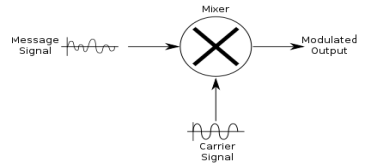


DSB-SC Modulator

DSB-SC is generated by a mixer. In its most common application, two signals are applied to a mixer, and it produces new signals at the sum and difference of the original frequencies. This consists of a message signal multiplied by a carrier signal. The mathematical representation of this process is shown below, where the product-to-sum trigonometric identity is used.

Vmcos(ωmt) X Vccos(ωct) = (VmVc/2) [cos((ωm + ωc)t)  +  cos((ωm - ωc)t)]

                                                                     (Modulated signal)

Where, Vmcos(ωmt) is the message signal

             Vccos(ωct)  is the carrier signal


Normal AM modulation vs DSB-SC

Normal AM modulation process is represented as

xAM(t) = Ac[1 + mx(t)]cosꞷct

where m is the modulation index

In case of AM Modulation carrier is modulated by varying amplitude linearly proportional to baseband signal.


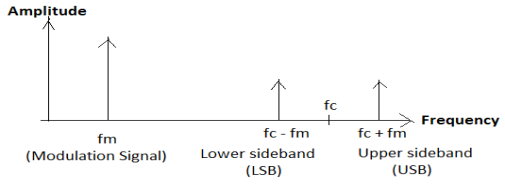
Theoretically, the amplitude-modulated wave has three frequencies. Those are carrier frequency fc, upper sideband frequency fc + fm, and lower sideband frequency fc - fm. After modulation, this signal in the frequency domain looks like this


We know the information is in sidebands. So there is no need to send only carrier frequency when it consumes 50% of the total transmitted power. This system will be more efficient when we send only a single sideband as sidebands containing identical copies of the same information and construct another sideband from the transmitted one. We basically follow this procedure in a single sideband suppressed carrier (SSB-SC) modulation process.


Efficiency of DSB-SC modulation

PAM  =  0.5Ac2  +  0.25m2Ac2

Where sidebands contain power 0.25m2Ac2 (say, Psb) and carrier frequency contains power 0.5Ac2 (say Pc).

In the case of DSB-SC we transmit sidebands and suppress the carrier. So, efficiency of a DSB-SC signal is calculated as

ղ = [Psb  / (Pc  +  Psb)]

   = [0.25m2Ac2  / (0.5Ac2  +  0.25m2Ac2)]  <  (1/3)

For AM, less than 33% of the power is in the sidebands. For DSB, 100% of the power is the sidebands.


DSB-SC Detector

For DSBSC, Coherent Demodulation is done by multiplying the DSB-SC signal with the carrier signal (with the same phase as in the modulation process) just like the modulation process. This resultant signal is then passed through a low pass filter to produce a scaled version of the original message signal.


(VmVc/2) [cos((ωm + ωc)t)  +  cos((ωm - ωc)t)] X Vc‘ cos(ωct)

= (1/2. Vc. Vc‘)Vm cos(ωmt) +  (1/4. Vc. Vc‘Vm) [cos((ωm + 2ωc)t)  +  cos((ωm - 2ωc)t)]

The equation above shows that by multiplying the modulated signal by the carrier signal, the result is a scaled version of the original message signal plus a second term. Since ωc >> ωm , this second term is much higher in frequency than the original message signal. Once the signal passes through a lowpass filter, the higher frequency component is removed, leaving the original message signal.


Q & A and Summary

Q1: What does DSB-SC stand for, and how does it differ from conventional AM?

DSB-SC stands for Double Sideband Suppressed Carrier. Unlike conventional Amplitude Modulation (AM), which transmits the carrier along with the sidebands, DSB-SC suppresses the carrier, transmitting only the sidebands. This results in more power efficiency and bandwidth utilization.

Q2: What is the mathematical expression for a DSB-SC modulated signal?

The DSB-SC signal \( s(t) \) is given by:
\( s(t) = A_c m(t) \cos(2\pi f_c t) \)
where \( A_c \) is the carrier amplitude, \( m(t) \) is the message signal, and \( f_c \) is the carrier frequency.

Q3: Why is the carrier not transmitted in DSB-SC?

The carrier does not contain useful information. Transmitting it would waste power. By suppressing the carrier, DSB-SC systems become more energy-efficient.

Q4: Explain the frequency domain representation of DSB-SC.

The frequency-domain representation is:
\( S(j\omega) = \frac{1}{2} \left[ M(j(\omega - \omega_c)) + M(j(\omega + \omega_c)) \right] \)
This shows that the message spectrum is shifted to both \( +\omega_c \) and \( -\omega_c \), creating upper and lower sidebands.

Q5: What is the role of a coherent detector in DSB-SC demodulation?

A coherent detector multiplies the received signal with a locally generated carrier that is in phase and frequency sync with the original. Any phase or frequency mismatch results in distortion of the demodulated signal.

Q6: What distortion occurs if synchronization is not perfect during demodulation?

Imperfect synchronization leads to phase or frequency mismatch. This results in signal distortion and loss of message fidelity during recovery.

Q7: Why is a Low Pass Filter (LPF) used after coherent detection?

After coherent detection, the product contains both baseband and high-frequency components (at double the carrier frequency). The LPF removes high-frequency components, isolating the original baseband message.

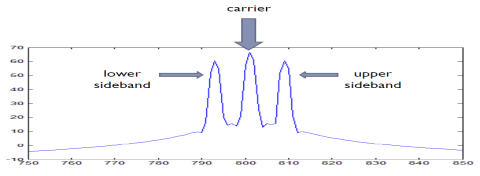
Q8: What happens in the frequency spectrum when a message signal is modulated using DSB-SC?

The spectrum of the message signal \( M(j\omega) \) is shifted to center around \( +\omega_c \) and \( -\omega_c \). This produces two symmetrical sidebands (USB and LSB) and the carrier is not present.

Q9: Can DSB-SC be demodulated without using the exact same carrier frequency?

No, DSB-SC requires exact carrier frequency and phase for coherent demodulation. Any deviation leads to inaccurate recovery of the message signal.

Q10: What are the key advantages and disadvantages of DSB-SC?

Advantages: Efficient use of power, better bandwidth usage.
Disadvantages: Requires complex coherent detection and exact carrier synchronization.


Further Reading

  1. Comparisons between DSB-SC and SSB-SC
  2. SSB-SC Modulation and Demodulation 
  3. DSB-SC in MATLAB

People are good at skipping over material they already know!

View Related Topics to


Contact Us

Name

Email *

Message *

Popular Posts

Constellation Diagrams of ASK, PSK, and FSK with MATLAB Code + Simulator

📘 Overview of Energy per Bit (Eb / N0) 🧮 Online Simulator for constellation diagrams of ASK, FSK, and PSK 🧮 Theory behind Constellation Diagrams of ASK, FSK, and PSK 🧮 MATLAB Codes for Constellation Diagrams of ASK, FSK, and PSK 📚 Further Reading 📂 Other Topics on Constellation Diagrams of ASK, PSK, and FSK ... 🧮 Simulator for constellation diagrams of m-ary PSK 🧮 Simulator for constellation diagrams of m-ary QAM BASK (Binary ASK) Modulation: Transmits one of two signals: 0 or -√Eb, where Eb​ is the energy per bit. These signals represent binary 0 and 1.    BFSK (Binary FSK) Modulation: Transmits one of two signals: +√Eb​ ( On the y-axis, the phase shift of 90 degrees with respect to the x-axis, which is also termed phase offset ) or √Eb (on x-axis), where Eb​ is the energy per bit. These signals represent binary 0 and 1.  BPSK (Binary PSK) Modulation: Transmits one of two signals...

Fading : Slow & Fast and Large & Small Scale Fading (with MATLAB Code + Simulator)

📘 Overview 📘 LARGE SCALE FADING 📘 SMALL SCALE FADING 📘 SLOW FADING 📘 FAST FADING 🧮 MATLAB Codes 📚 Further Reading LARGE SCALE FADING The term 'Large scale fading' is used to describe variations in received signal power over a long distance, usually just considering shadowing.  Assume that a transmitter (say, a cell tower) and a receiver  (say, your smartphone) are in constant communication. Take into account the fact that you are in a moving vehicle. An obstacle, such as a tall building, comes between your cell tower and your vehicle's line of sight (LOS) path. Then you'll notice a decline in the power of your received signal on the spectrogram. Large-scale fading is the term for this type of phenomenon. SMALL SCALE FADING  Small scale fading is a term that describes rapid fluctuations in the received signal power on a small time scale. This includes multipath propagation effects as well as movement-induced Doppler fr...

Online Simulator for ASK, FSK, and PSK

Try our new Digital Signal Processing Simulator!   Start Simulator for binary ASK Modulation Message Bits (e.g. 1,0,1,0) Carrier Frequency (Hz) Sampling Frequency (Hz) Run Simulation Simulator for binary FSK Modulation Input Bits (e.g. 1,0,1,0) Freq for '1' (Hz) Freq for '0' (Hz) Sampling Rate (Hz) Visualize FSK Signal Simulator for BPSK Modulation ...

Theoretical BER vs SNR for BPSK

Theoretical Bit Error Rate (BER) vs Signal-to-Noise Ratio (SNR) for BPSK in AWGN Channel Let’s simplify the explanation for the theoretical Bit Error Rate (BER) versus Signal-to-Noise Ratio (SNR) for Binary Phase Shift Keying (BPSK) in an Additive White Gaussian Noise (AWGN) channel. Key Points Fig. 1: Constellation Diagrams of BASK, BFSK, and BPSK [↗] BPSK Modulation Transmits one of two signals: +√Eb or −√Eb , where Eb is the energy per bit. These signals represent binary 0 and 1 . AWGN Channel The channel adds Gaussian noise with zero mean and variance N₀/2 (where N₀ is the noise power spectral density). Receiver Decision The receiver decides if the received signal is closer to +√Eb (for bit 0) or −√Eb (for bit 1) . Bit Error Rat...

What is - 3dB Frequency Response? Applications ...

📘 Overview & Theory 📘 Application of -3dB Frequency Response 🧮 MATLAB Codes 🧮 Online Digital Filter Simulator 📚 Further Reading Filters What is -3dB Frequency Response?   Remember, for most passband filters, the magnitude response typically remains close to the peak value within the passband, varying by no more than 3 dB. This is a standard characteristic in filter design. The term '-3dB frequency response' indicates that power has decreased to 50% of its maximum or that signal voltage has reduced to 0.707 of its peak value. Specifically, The -3dB comes from either 10 Log (0.5) {in the case of power} or 20 Log (0.707) {in the case of amplitude} . Viewing the signal in the frequency domain is helpful. In electronic amplifiers, the -3 dB limit is commonly used to define the passband. It shows whether the signal remains approximately flat across the passband. For example, in pulse shapi...

Pulse Shaping using Raised Cosine Filter (with MATLAB + Simulator)

  MATLAB Code for Raised Cosine Filter Pulse Shaping clc; clear; close all ; %% ===================================================== %% PARAMETERS %% ===================================================== N = 64; % Number of OFDM subcarriers cpLen = 16; % Cyclic prefix length modOrder = 4; % QPSK oversample = 8; % Oversampling factor span = 10; % RRC filter span in symbols rolloff = 0.25; % RRC roll-off factor %% ===================================================== %% Generate Baseband OFDM Symbols %% ===================================================== data = randi([0 modOrder-1], N, 1); % Random bits txSymbols = pskmod(data, modOrder, pi/4); % QPSK modulation % IFFT to get OFDM symbol tx_ofdm = ifft(txSymbols, N); % Add cyclic prefix tx_cp = [tx_ofdm(end-cpLen+1:end); tx_ofdm]; %% ===================================================== %% Oversample the Baseband Signal %% ===============================================...

Understanding the Q-function in BASK, BFSK, and BPSK

Understanding the Q-function in BASK, BFSK, and BPSK 1. Definition of the Q-function The Q-function is the tail probability of the standard normal distribution: Q(x) = (1 / √(2π)) ∫ x ∞ e -t²/2 dt What is Q(1)? Q(1) ≈ 0.1587 This means there is about a 15.87% chance that a Gaussian random variable exceeds 1 standard deviation above the mean. What is Q(2)? Q(2) ≈ 0.0228 This means there is only a 2.28% chance that a Gaussian value exceeds 2 standard deviations above the mean. Difference Between Q(1) and Q(2) Even though the argument changes from 1 to 2 (a small increase), the probability drops drastically: Q(1) = 0.1587 → errors fairly likely Q(2) = 0.0228 → errors much rarer This shows how fast the tail of the Gaussian distribution decays. It’s also why BER drops drama...

BER vs SNR for M-ary QAM, M-ary PSK, QPSK, BPSK, ...(MATLAB Code + Simulator)

📘 Overview of BER and SNR 🧮 Online Simulator for BER calculation of m-ary QAM and m-ary PSK 🧮 MATLAB Code for BER calculation of M-ary QAM, M-ary PSK, QPSK, BPSK, ... 📚 Further Reading 📂 View Other Topics on M-ary QAM, M-ary PSK, QPSK ... 🧮 Online Simulator for Constellation Diagram of m-ary QAM 🧮 Online Simulator for Constellation Diagram of m-ary PSK 🧮 MATLAB Code for BER calculation of ASK, FSK, and PSK 🧮 MATLAB Code for BER calculation of Alamouti Scheme 🧮 Different approaches to calculate BER vs SNR What is Bit Error Rate (BER)? The abbreviation BER stands for Bit Error Rate, which indicates how many corrupted bits are received (after the demodulation process) compared to the total number of bits sent in a communication process. BER = (number of bits received in error) / (total number of tran...