Ray tracing Method

 

Ray tracing Method

Because of its advantages in industry, wireless networking is increasingly growing to new heights, with the ability to provide high-speed information sharing between handheld devices anywhere in the globe. Any empirically based radio propagation model is useful for a specific application. We can't adapt a model developed for one application to another, and these models lack the generality and ease of use that a simple theoretical formulation provides. As a result, deterministic models that can be used to various conditions without affecting the precision. It is basically based on EM wave propagation characteristics.

Reflection and transmission

Dielectric Boundary:

For radio wave propagation, the physical properties of the walls and other materials for which it reflect and scatter radio waves are determined by boundary conditions. In practise, specifying information with precision less than the wavelength is impractical in dynamic environments. Ray tracing (site-specific model) has emerged as the dominant approach for determining propagation in such environments to solve this problem. Furthermore, wireless network administrators may use ray tracing to see the impact of signals as they bounce off walls inside the building. Because of the widespread use of indoor wireless networks, there has been an increasing interest in propagation estimation for indoor environments over the last two decades.

Snell’s Law of Reflection:

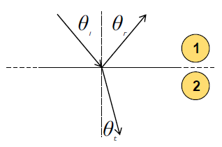
Where, θ_i = Incidence Angle

θ_r = Reflection Angle

θ_t = Transmission / refraction Angle

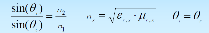
The rays of light (EM-waves) travel the direction of stationary optical length, according to Fermat's theory (principle of least time). According to Snell's theorem, the reciprocal proportion of the indices of refraction is proportional to the proportion of the sines of the angles of incidence and refraction.

(8.3)

η = refractive index; ε= permitivity; μ= permeability

Fresnel Reflection Coefficients:

The usual vector to the refelecting surface and the incedence wave's poynting vector form the plane of incedence (parallel or parpendicular).

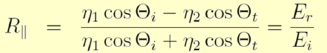
Fresnel parallel reflection coefficient:

………………(8.4)

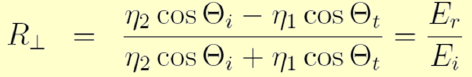
Fresnel perpendicular reflection coefficient:

………………(8.5)

Where, 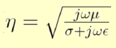 , ω= angular frequency. So, fresnel coefficient is frequency dependent.

Perfect Electric Conductor (PEC):

PEC indicates such a codition where reflection is possible but further transmission is not possible.

Orthogonal PEC reflection:

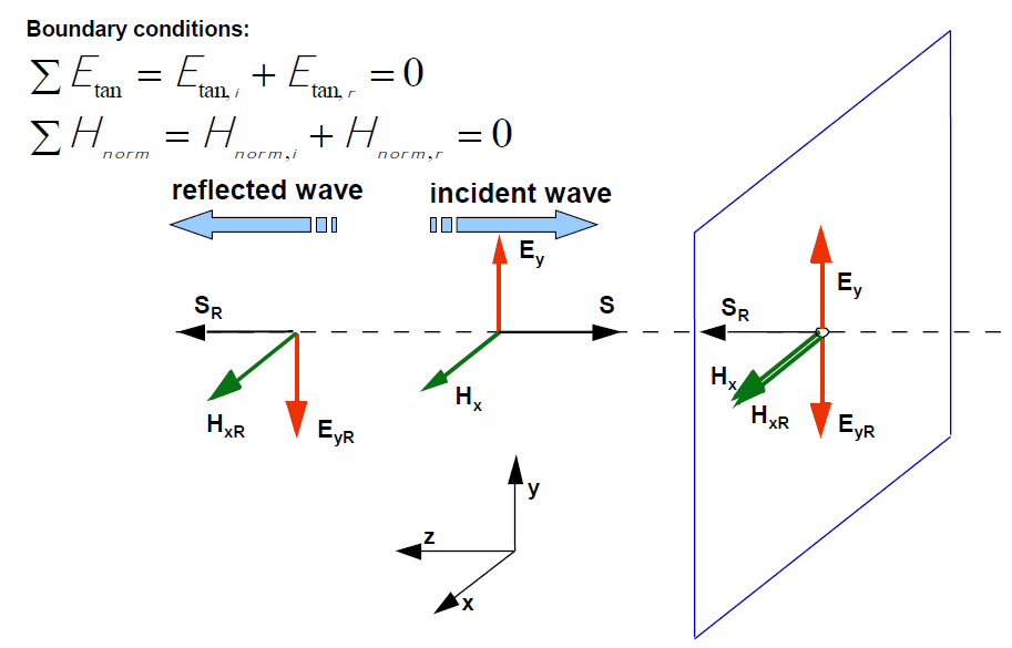
Fig 8.6: Illustration of perfect conductor bounderies

Here E_tan = tansential component of electric field and i & r denotes the incedence and reflection, repectively

For PEC reflection:

Parallel Fresnel Reflection coefficent, R_|| or Γ_|| = +1

Perpendicular Fresnel Reflection coefficent, R_⊥ or Γ_⊥ = -1

Fresnel coefficient in case of diffraction:

The ellipsoid that defines the nth Fresnel zone is bounded by a Tx-Rx path that is N half wavelengths longer than the direct Tx-Rx path dT + dR between Tx and Rx.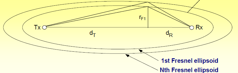 

Fig 8.7: Illustration of fresnel zone using two ray propagation method

Where,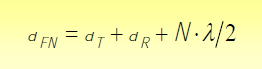 

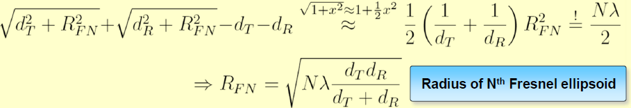
(8.6)

In the above equation, assuming the distance d_T and d_R are more larger than the radius. We take the roots in series. And retain first two term for simplicity in calculation. Then, we predict pathloss according to the distance of total path length (Younis, 2003).

The Geometrical Optics (GO) theory is used to treat plane surface reflections and transmissions in the ray tracing method. The so-called ray assumptions in geometrical optics assume that wavelengths are too short in comparison to the dimensions of the obstacles (here it is wall). These high-frequency radio waves have the same properties as light waves. As a result, ray propagation can be used to model signal propagation. Reflection and propagation theory focused on Fermat's theorem and Fresnel coefficient may be used to model the interaction of rays with partitions inside buildings. According to Fermat's theorem, a ray follows the direction that takes the least amount of time, and occurs only when the angle of incidence is identical to the angle of reflection or propagation.

Ray tracing method:

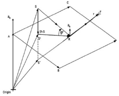
Fig 8.8: An illustration of first order reflection (Sidhu, 2012)

To evaluate the distance of the normal line's end point from origin, the transmitter, say T, to a building wall (here the reflective wall is represented by a plane), a single reflection is required from transmitter to reflective wall. Following reflection, the distance between T and the plane (wall) is doubled, and the point at the end of the doubled line is referred to as an image (T') here. All required planes to calculated reflected paths, can be created based on the images of a source object. Let assume, N is the total number of planes, then source (here the transmitter) would have N number of first-order reflections, N(N – 1) number of second order reflection images, and N(N – 1) number of third order reflections, and so on. Each node in the above figure represents a scenario object (intervening walls, a building wall, the receiver antenna, etc), with branches representing line of sight links between two node, where the number of first order reflection will be N-fold and then including second order reflection total reflection will be N – 1 fold. Connecting the source point (T), the reflection point (R), and the receiver point (R) yields the direction of only single reflection propagation (F) due to a single plane, P. Then the position of the reflection point R on plane P is determined by first determining the image of the source object in the plane, which is defined as T", and then we have to determine the intersection point on plane P and the vector distance from image T" to F. The plane has the following definition:

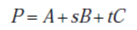 (i)

where A is the plane's distance from the origin, defined by [0 0 z], B and C are the ceiling's [x 0 0] and [0 y 0], respectively, and s and t are the spatial co-ordinates. T' is calculated as the perpendicular projection point of T on the plane, and the relationship between T and T' is expressed by

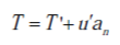 (ii)

where u’ is the displacement along the unit vector as shown and a_n is unit vector normal to the plane denoted as

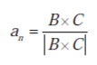 (iii)

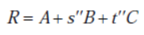
position vectors for projection point T’ can be represented as

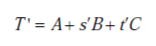(iv)

Substituting (iv) into (ii),

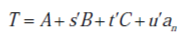 (v)

 (vi)

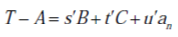
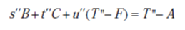
Rearranging Equation (v) in matrix form:

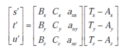 (vii)

To measure the position vector T', substitute into (ii) until (vii) is solved for u'. The representation of the source point in the plane is denoted by

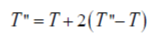 (viii)

R's position can be expressed in the following way:

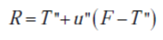 (ix)

 (x)

Rearranging (ix) and (x),

 (xi)

Equation (xi) expressed in matrix form is

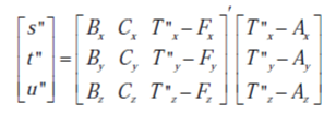 (xii)

The reflection point R is then found by substituting u" into (ix). This procedure is repeated for each wall or partition in the scenario.

The Fresnel Reflection Coefficients (Γ) are used to measure reflections and signals across walls and partitions. The perpendicular or parallel Fresnel Reflection Coefficients are used depending on the polarisation of the wave relative to the interface, which is denoted by

Γ_|| =  θ_i η₁ θ_t η₂ (η₁cos θ_i - η₂cos θ_t) / (η₁cos θ_i + η₂cos θ_t) = E_r / E_i

Γ_⊥ =  θ_i η₁ θ_t η₂ (η₂cos θ_i - η₁cos θ_t) / (η₂cos θ_i + η₁cos θ_t) = E_r / E_i (xiii)

The necessary coefficients are multiplied by the field vector as shown in equation (xiv) below. For the i^th ray, the multiple reflection signal intensity at the receiver is given by

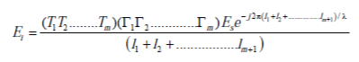 (xiv)

Where, E_i = Multiple reflection signal strength at Receiver

l₁+l₂+… +l_k = Total reflection distance, k any positive integer

Γ_­1, Γ₂, …, Γ_k = Coefficients of reflection at reflection points 1, 2,..., m

T₁, T₂, …, T_n = Coefficients of transmission at each wall or partition 1, 2,..., n

(Sidhu, 2012)

The fields for multi-paths or each of the n rays arriving at the receiver form the corresponding field vector at the receiver point. The vector number of field strengths determined resultant value of all rays arriving at receiver. The measurement of total electric field strength E_T is denoted as,

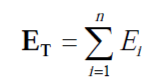 ………………………………………………………………(8.7)

Following the calculation of field strength, other parameters such as obtained power and path loss are determined.

In wireless communication, antenna aperture is a critical antenna parameter.

The potential to collect power from an incoming wave is known as antenna aperture or effective aperture. If a power density, S of 1 mW/m² exists and an antenna picks up 1 mW of power, it is as if the antenna harvested the power over a 1 m² coverage. Gain, g (say), and working wavelength all influence effective aperture.

 ……………………………….(8.8)

Here, gain, g in the power ratio

Wavelength, λ = c₀/f

c₀ =speed of light in free space;

f=frequency

Gain g in dB= 10log₁₀(g)

P_r = A_e * S; where, A_e= effective aperture, S= power density of the incoming wave

………………………….(8.9)

Where, E= E (measured in V/m) is the strength of electric field.

H= H (measured in A/m) is the strength of magnetic field.

Z₀=characteristic impedance of vacuum that is 377 ohm (approx.)

From electric field strength , magnetic field strength, operating frequency and antenna aperture we can calculate the received power from the equations mentioned above.