UWB and mm-Wave Indoor Communication

UWB and mm-Wave Indoor Communication

8.1. Introduction:

Higher frequency bands are intended for wireless and wired broadband networks. Since it allows for more spectrum coverage and higher bandwidth demands. To ensure that a wireless communication device performs well, it is essential to define the radio transmission channel. Wireless communication is also becoming popular in industrial operation day by day. It is needed to control appliances i.e, automated vehicles, machine to machine communication in factories, etc. compare to wired communication, and wireless communication is cost efficient. Fifth generation (5G) technology has gathered a great interest in industrial operation due to its low reliable latency. Industrial applications need more careful evaluation. Industrial environment faces a great quantity of reflective metal surfaces. So it is required to develop a suited physical layer for this particular environment.

Indoor residential: This environment is suitable for home networking. There may be different appliances, sensors for detecting fire, smoke, etc, within a small area.

Indoor office: office rooms are usually comparable in size to residential areas. Other rooms i.e, laboratories, etc, are larger. Most offices are linked by corridors. Office rooms contains bookshelves, furniture, thin office partitions, etc. They add extra attenuation.

Industrial environment: it usually contains large number of machineries. It leads metallic reflection. So, here severe multipath is produced.

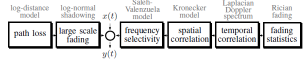
Fig 8.1: Components for indoor industrial communication

Small small fading occurs due to multipath, different angle of arrival/ departure (AOA/ AOD), etc. Small scale fading is responsible for frequency selective behaviour of channel and temporal correlation as shown in figure 8.1.

Pathloss:

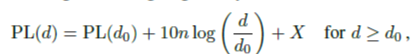
Pathloss, shadowing is categorized with large scale fading. Signal power decreases over distance, is called pathloss.

………………………(8.1)

Here, d₀= reference distance (usually 1 m)

n = pathloss exponent

X= standard deviation in dB

8.2. Ultra wideband Wireless Communication:

Ultra wideband communication are suitable for short range communication. It transmits narrow impulses ranges up to picoseconds. So it achieves wide spectrum. Sometimes duty cycles of UWB rectangular impulses are kept in less than 1%. On the other hand we allocate very low signal power (figure 8.2) that it cannot interface much with other signals of operating over those frequencies and obviously, it is suitable for short range communication. As impulses are very narrower so it helps us to achieve positioning accuracy up to 5-10 centimetres. It can track the location of devices or objects in real time (Frenzel, 2007).

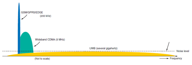
Fig 8.2: UWB signal bandwidth compared to conventional and spread spectrum signal bandwidth (Frenzel, 2007).

UWB was invented in 1960. On that time it was known as impulse baseband wireless. But now it is growing interest in short ranging communication because of its positioning accuracy and low power short range communication.

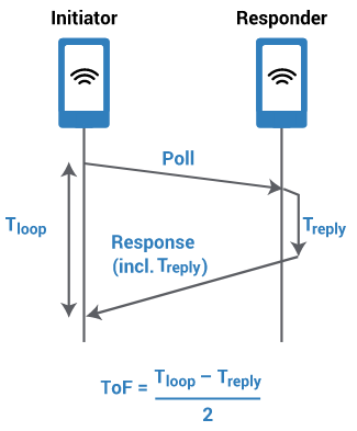
Fig 8.3: Ranging between two UWB enabled devices

Here is above figure 8.3, it is illustrated that when two UWB enabled devices come closer or come in range they start ranging. The ranging is done by time of flight (ToF) time which indicates time required to perform a round trip of packets between initiator and responder devices. As pulses are very narrower in UWB communication then it can give us high positioning accuracy to track a device’s location in real time and enable communication more reliable. It can also measure angle of arrival and angle of departure at antenna boresight calculating the phase differences between antenna elements.

8.3. Small scale fading channel model:

Rapid changes in recived signal i.e, due to angle of arrival and departure (AOA and AOD), multipath, doppler frequency shift etc are termed as small scale fading. In industrial environment small scale fading can be modelled as Rician fading. The ratio of dominant component signal power to scattered multi-path component signal power is used to measure the Rician k-factor.

1. Frequency selectivity:

In a wireless communication signal reaches from transmitter to receiver with different path lengths. Signal multipaths (MPCs) which arrives at receiver at same time is denoted as tap. Here communication channels is linear, time-variant (LTV), and causal.

………………………(8.2)

Here, y(t)= received signal

x(t)= transmitted signal

x(t-τ)= x(t) signal delayed by propagation delay τ

h(t, τ)= time-variant impulse response of radio channel

Factor h(t, τ) can represented as infinite sum of taps. In practical, h(t, τ) is derived from limited number of taps (Let U),

Here, i^th tap for propagation delay τ_i , and tap h(t, τ)’s amplitude and phase shift

Further, h(t, τ) can be divided into complex vector c_i (t) and mean path amplitude β_i . c_i (t) is time dependent complex factor for stochastic fading process.

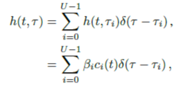
Fig 8.4: Saleh Valenzuala (SV) model assumptions

Saleh Valenzuala (SV) model is widely accepted model for indoor wireless communication. Here, MPCs arrive in group, is considered as clusters. Arrival time of l-th cluster denoted as T_l here in above figure 8.4. Each cluster contains number of rays or taps. Similarly, k^th tap in l^th cluster denoted as τ_kl .

2. Spatial and temporal correlation:

For multi-antenna system spatial correlation occurs. It improves the system performance. In case of MIMO communication transmission between each tx and rx pairs are statistically independent. So communication channel become more reliable (decreases the bit error rate). Spatial correlation can be interpreted as signal’s correlation in spatial direction. Due to multipath propagation signal reaches at receiver at different delay time but they are correlated (linear in nature). Specially, for indoor communication multipath are characterized by different clusters (taps) , but mean AOAs (angle of arrivals) are uniformly distributed for different clusters. When antennas (either tx or rx, or both) are moving, doppler shift is produced. Then channel variation over time is called Doppler power density spectrum. A bell shaped Doppler spectrum is commonly used for WLAN channel models. For example an static transmitter and an moving receiver can design the Doppler spectrum for a particular scenario (Traßl, 2019).

Modified Saleh-Valenzuala Model:

• Arrival of paths in clusters

• Arrival of clusters and rays follows mixed poission distribution for any arrival time

• NLOS environments have first increase, then decrease of power delay profile.

Poission Distribution:

It is a discrete probability distribution function that represents the probability of a certain set of occurring events. Events are said to occur in a fixed interval of time or space if they occur at a known constant mean rate and regardless of the time after the previous occurrence

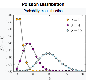
Fig 8.5: k indicates number of occurrences of events and expected rate of occurrences is denoted by λ

The number of MPC arrivals λ in any delay interval of length T after the arrival of the first MPC is Poisson distributed with mean, λ i.e.,

Probability, P = (λ T)^k e^{- λ T} / k! ; where k=events in interval T

λ=mean arrival rate of MPCs

Here in the above saleh-valenzuala model, average mean= β, cluster rate is Γ and ray (in each cluster) rate is λ (Meijerink, 2014).