Design of 8-bit Synchronous Counter

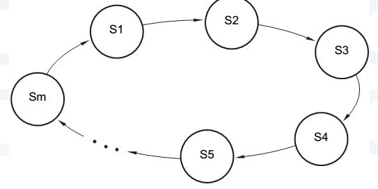
A counter is a sequential circuit that counts pulses and is widely used for event counting, frequency division, timing, and control operations. Its outputs progress in a predictable repeating pattern, advancing one state per clock pulse. The modulus (m) of a counter is the number of states in its cycle. A counter with m states is called a modulo-m or divide-by-m counter.

Fig.1: General Structure of a counter’s state diagram—a single cycle

Ripple Counters

An n-bit binary counter can be constructed using n flip-flops. Each bit toggles when the preceding bit changes from 1 to 0, generating a carry to the next higher-order bit. This “rippling” of the carry gives the ripple counter its name.

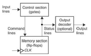
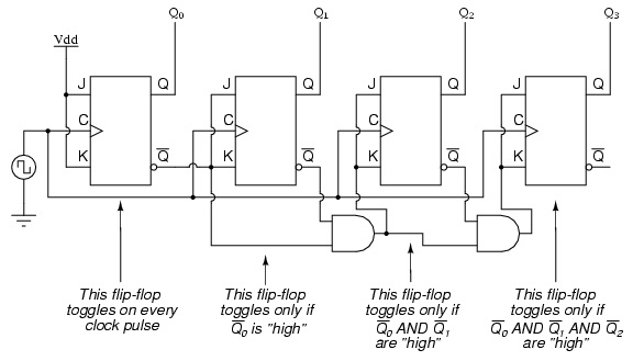
Synchronous Counters

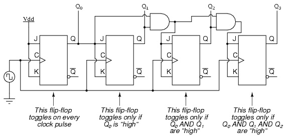
Unlike ripple counters, synchronous counters have all flip-flop clock inputs connected to the same CLK signal, so all outputs change simultaneously after a single flip-flop propagation delay. T flip-flops with enable inputs are used, and combinational logic determines which flip-flops toggle per clock cycle.

Fig.2: A synchronous 4-bit binary counter with serial enable logic

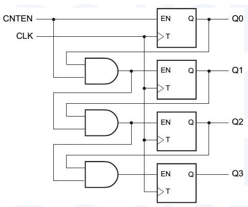
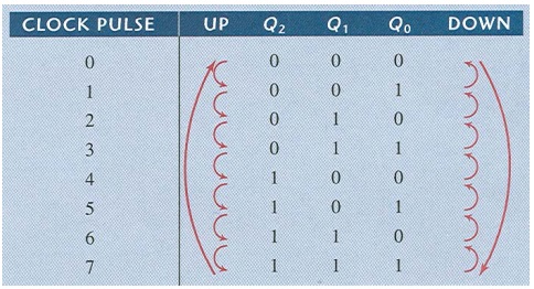
Master count enable signal (CNTEN) allows each flip-flop to toggle only when asserted and all lower-order bits are 1. Counters can operate in two directions:

• UP – count from MSB to LSB
• DOWN – count from LSB to MSB

Fig.3: Synchronous Counters

Fig.4: Circuit Diagram of 4-bit Up Counter

Fig.5: Circuit Diagram of 4-bit Down Counter

Fig.6: Example of 3-bit Up & Down Counting Process

Circuits / Block Diagrams

Fig.7: Block Diagram of Up Counter

Fig.8: Internal Circuit of Up Counter

Fig.9: Block Diagram of Down Counter

Fig.10: Internal Circuit of Down Counter

Observations & Data

Write a VHDL program, run it to generate the RTL schematic, and then create the Test Bench Waveform (TBW). The input and output waveforms can then be observed according to the given inputs.

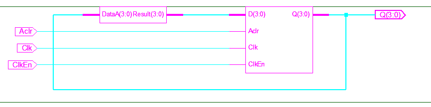
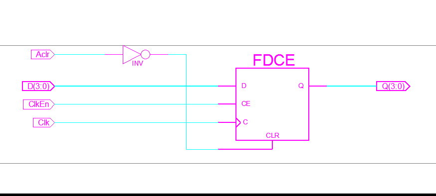
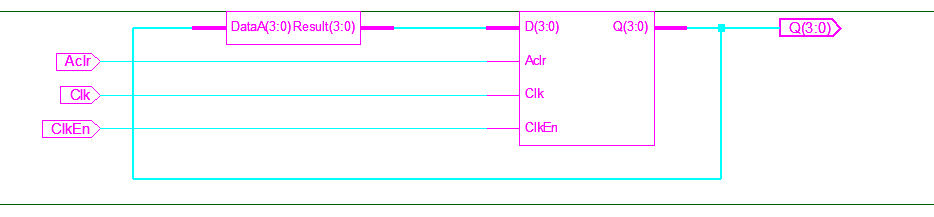
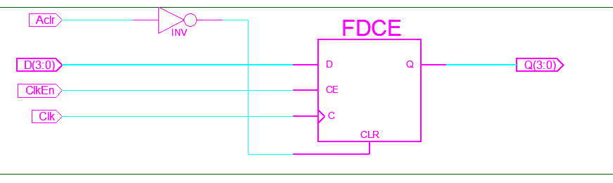
RTL Schematic

[Include RTL schematic image]

Test Bench Waveform (TBW)

[Include TBW waveform image]

Input & Output Waveform

[Include waveform image]

Procedure

Refer to Xilinx Software Procedure for step-by-step VHDL simulation and synthesis.

Conclusion

Using Xilinx ISE software, the VHDL program was implemented, RTL schematic generated, and Test Bench Waveform obtained. The input/output waveforms matched the expected design, demonstrating correct synchronous counter operation.