LDPC Encoding and Decoding Techniques

Low Density Parity Check (LDPC) Guide

Comprehensive analysis of linear error-correcting block codes, Tanner graphs, and 5G-NR implementations.

📘 Overview 🧮 Encoding 🧩 Decoding 📚 Resources

Theory Encoding Tech Tanner Graph 5G Encoding Decoding

'LDPC' is the abbreviation for 'low density parity check'. LDPC code H matrix contains very few amount of 1's and mostly zeroes.

LDPC codes are error correcting code. Using LDPC codes, channel capacities that are close to the theoretical Shannon limit can be achieved.

Low density parity check (LDPC) codes are linear error-correcting block code suitable for error correction in a large block sizes transmitted via very noisy channel. Applications requiring highly reliable information transport over bandwidth restrictions in the presence of noise are increasingly using LDPC codes.

1. LDPC Encoding Technique

The proper form of H matrix is derived from the given matrix by doing multiple row operations as shown above.

In the above, H is parity check matrix and G is generator matrix. If you consider matrix H as [-P' | I] then matrix G will be [Ik | P], where P' is the transpose of P and Ik is the identity matrix of size k by k.

Then the codeword is generated by doing mod 2 multiplication of G times of the message bit string

For example, codeword for bit string '101' is obtained by ( 1 0 1 ) mod 2 multiplication G = ( 1 0 1 0 1 1 )

1.1. Tanner Graph

H * C' = 0
c1 Å c2 Å c3 Å c4 = 0
c3 Å c4 Å c6 = 0
c1 Å c4 Å c5 = 0

H (mod 2 multiplication) r = H (mod 2 multiplication) (c + e)
H (mod 2 multiplication) c = 0
H (mod 2 multiplication) e = error

In the above discussion, the H matrix is not really a low density parity check matrix or sparse matrix. There are some procedure to form a sparse H matrix.

Contents

• • Introduction
• • LDPC codes
• • Regular and irregular LDPC codes
• • Tanner graph representation
• • Non-binary LDPC Codes
• • Encoding of LDPC codes in the 5G standard
• • System model
• • Summary
• • References

Introduction

Low-density parity-check (LDPC) code is a class of linear block code, a method of transmitting a message over a noisy transmission channel. It is a capacity-approaching code. Now a days, non-binary low-density parity-check (LDPC) codes have attracted much attention because of noticeable performance. It has excellent performance for high-spectral efficiency transmission. We know mobile data demand is increasing day by day. Usually mobile data traffic increases 1000 fold over decades. Now, 5G is able to support terminal speeds of up to 300 km/h for vehicle-to-vehicle (V2V) and vehicle-to-infrastructure systems due low latency in the air. We adapt different coding techniques to improve network throughput. LDPC codes are constructed using sparse tanner graph. Binary LDPC code has been suggested by 3rd Generation Partnership Project (3GPP) enhanced mobile broadband (eMBB) in 5G. Non-binary LDPC codes are linear block codes dened over high-order finite field GF(q), where q> 2.

LDPC

LDPC (lower density parity check matrix) is a class of linear block code. ‘Low density’ refers to the characteristics of parity check matrix which contains only few ‘1’ in compare with ‘0’s. LDPC codes are arguably the best correction codes in existence at present time. LDPC codes are first introduced by R.Gallager in his Ph.D thesis in 1960 and soon forgotten due to introduction of reed Solomon codes and the implementation issues due to technical knowhow at that time.

We can define N bits long LDPC code in terms of M numbers of parity check equations and dropping those parity check equations with M X N parity check matrix H

$$H = \begin{bmatrix} 1 & 1 & 0 & 1 & 0 & 0 \\ 0 & 1 & 1 & 0 & 1 & 0 \\ 1 & 0 & 1 & 0 & 0 & 1 \end{bmatrix}$$

Where, H is 3 by 6 parity check matrix; Columns 4th, 5th and 6th contains parity bits; M=number of parity check equations; N= number of bits in the code word

Regular and irregular LDPC codes

In regular LDPC codes the number of ‘1’s in any row of parity check matrix (H) will be equal and applies to the column also. In case of irregular LDPC codes number of ‘1’s will be different in rows and columns of parity check matrix.

$$H = \begin{bmatrix} 1 & 1 & 0 & 0 & 1 & 0 \\ 1 & 0 & 0 & 1 & 0 & 1 \\ 1 & 1 & 1 & 0 & 0 & 1 \end{bmatrix}$$

Here, H is 3 by 6 irregular LDPC parity check matrix. Now, I am considering a 6 bit long codewords in the form of C=[ c1 c2 c3 c4 c5 c6 ]. We know, HCT = 0

• • \(\begin{bmatrix} 1 & 1 & 0 & 0 & 1 & 0 \\ 1 & 0 & 0 & 1 & 0 & 1 \\ 1 & 1 & 1 & 0 & 0 & 1 \end{bmatrix}\ \lbrack c1\ c2\ c3\ c4\ c5\ c6\rbrack T\)
• • C1 ⊕ c2 ⊕ c5 = 0;
• • C1 ⊕ c4 ⊕ c6 = 0;
• • C1 ⊕ c2 ⊕ c3 ⊕ c6= 0;

The parity check matrix defines a rate, R= k/n for (n, k) code where k= n-m. Codewords is said to be valid if it satisfies the syndrome calculation equation, CHT = 0. Codewords can be generated by multiplying message (M) with generator matrix G, C=M*G. G= [ I |PT] ; where H =[ p | I] ; I = identity matrix

Tanner graph representation

Tanner graph is a graphical representation of parity check matrix specifying parity check equations. Let a Tanner graph contains N(=6) number of variable nodes and M(=3) number of check nodes. In tanner graph mth check node is connected to nth variable node if and only nth element in in mth row , hmn in parity matrix H is ‘1’.

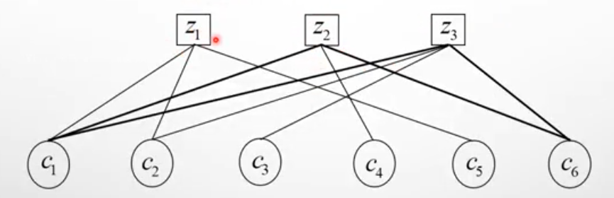
Fig: Tanner graph representation of 3 check nodes z1, z2, z3 and six variable nodes c1, c2, c3, c4, c5, and c6.

C1 ⊕ c2 ⊕ c5 = 0;
C1 ⊕ c4 ⊕ c6 = 0;
C1 ⊕ c2 ⊕ c3 ⊕ c6= 0;

Advantages of LDPC codes:

1. Perform close to Shannon limit capacity
2. High throughput
3. Very low bit error rate (BER)

Application of LDPC codes

1. Used in 10 GBIT Ethernet copper (10GBASEE-T) standard, which requires a high code rate.
2. Used in MIMO applications
3. Used in satellite communication

Non-binary LDPC Codes

Let GF(q), where q>2, is finite field with q element, (1, α, α2,…., αq-1); where, where q is a power of a prime and is a primitive element of GF(q). A q-ary LDPC code C of length N and dimension K is given by the null space of a sparse MXN matrix, where M= number of parity check equations. Code word C=[c0, c1 ,c2…c N-1]. We know, CHT= 0; where all operations of multiplication and addition all are defined over GF(q).

If H consists of circular permutation matrices (CPMs) of the same size over GF(q), then the null space over GF(q) of H gives a non-binary QC-LDPC code over GF(q). A graph's girth is defined as the minimum cycle length and denoted by g.

Construction of prime field based non-binary LDPC Codes:

The adjacent matrix A of matrix H over GF(q) can be obtained by replacing the nonzero entries of H with 1. Let p be a prime number and Fp is a prime field, p>2.

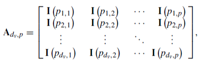
Where, I (p i,j) stands for a pXp CPM. Where for 1≤ I ≤ dv , 1≤ I ≤ dc , p i,j = (i-1)(j-1) (mode p). Where dv= column weight of LDPC matrix H, dc=row weight of LDPC matrix H

Masked Prime Field Based non-binary QC-LDPC Codes:

The main purpose of doing the process is to optimize short cycle distribution of QC-LDPC code. Because, Girth and the number of shortest cycles play important roles in the nonbinary LDPC code design. That process is called masking.

Encoding of LDPC codes in the 5G standard

Here, I will discuss couple of simple ways of encoding using parity check matrix. Small example: there is a code of parity check matrix let for (6, 3) code

$$H = \begin{bmatrix} 1 & 1 & 0 & 1 & 0 & 0 \\ 0 & 1 & 1 & 0 & 1 & 0 \\ 1 & 0 & 1 & 0 & 0 & 1 \end{bmatrix}$$

m = [m1 m2 m3]; C= [m1 m2 m3 p1 p2 p3]. Where, p1, p2, and p3 are parity bits. H matrix tells us H times C transpose: HCT= 0

$$\begin{bmatrix} 1 & 1 & 0 & 1 & 0 & 0 \\ 0 & 1 & 1 & 0 & 1 & 0 \\ 1 & 0 & 1 & 0 & 0 & 1 \end{bmatrix}\begin{bmatrix} m1 \\ m2 \\ m3 \\ p1 \\ p2 \\ p3 \end{bmatrix} = 0$$

There are 3 equations. Row 1: m1 ⊕ m2 ⊕ p1=0; Row2: m2⊕m3⊕p2=0; Row 3: m1⊕ m3⊕p3=0. So, p1 equals to m1⊕m2; P2= m2⊕m3; P3= m1⊕m3. We know H=[p|I]

$$P = \begin{bmatrix} 1 & 1 & 0 \\ 0 & 1 & 1 \\ 1 & 0 & 1 \end{bmatrix}$$

[p | I] [ mT pT ]T= 0 => Pm T + PT = 0 => PT = Pm T. [ p1 p2 p3]T = [P] [m1 m2 m3]T. Here, P is parity check matrix.

In fact, encoding of LDPC codes in the 5G standard also uses the same principle. If message bits are given and we use parity check matrix to compute the parity bits from the message bits.

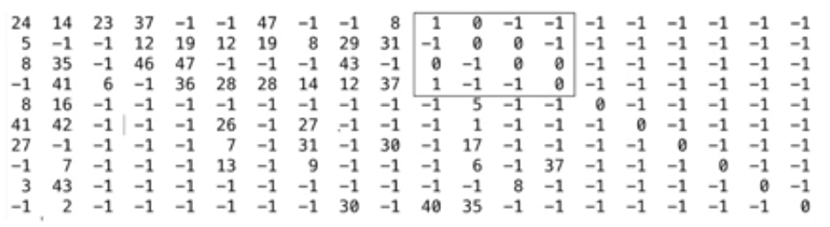
Let, B = base matrix in 5G, with an expansion factor of 5

$$B = \begin{bmatrix} 1 & 1 & 3 & 1 & 0 & - 1 \\ 2 & 0 & - 1 & 0 & 0 & 0 \\ 1 & 4 & 2 & 1 & - 1 & 0 \end{bmatrix}$$

Each entry -1 to 4, expansion factor 5 and each entry is replaced by a 5X5 matrix binary. -1 is replaced by all zero matrix and other number, say 0 or 1 or 2 or 3 or 4, is replaced by 5X5 identity matrix, column shifted, column rotate shifted that many times to the right. Element B1,1, B1,2, …B6,6, all are replaced by 5X5 identity matrix.

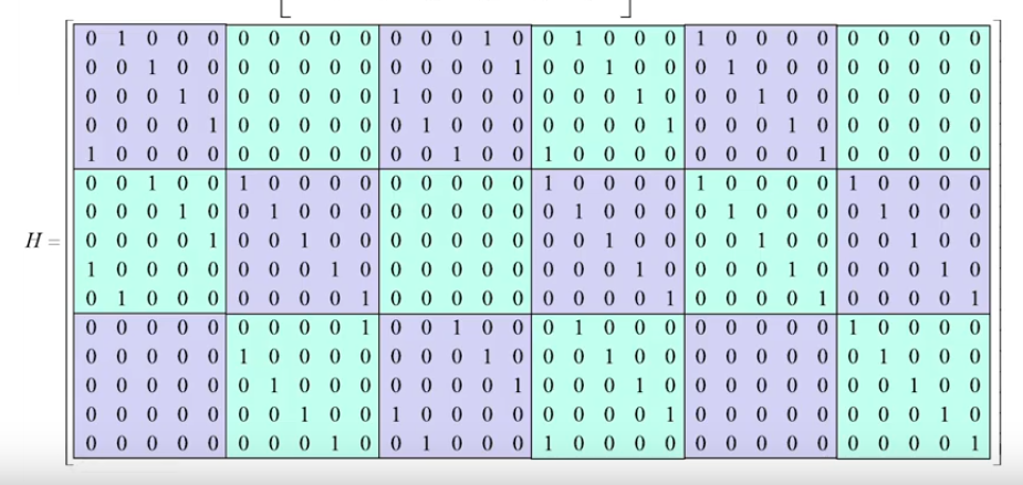
For base matrix 10X20, with expansion factor of 48 shown below:

Where, column 1 to 10 are message vectors, m=[m1 m2 m3….m10]; mi = 48 bits. Here, in the above figure we can see double diagonal identity matrix structure. Let an double diagonal matrix of expansion 5

$$H = \begin{bmatrix} I1 & 0 & I3 & I1 & I2 & I & 0 & 0 \\ I2 & I & 0 & I3 & 0 & 0 & I & I \\ 0 & I4 & I2 & I & I1 & 0 & I & I \\ I4 & I1 & I & 0 & I2 & 0 & 0 & I \end{bmatrix}$$

Here, 0= 5X5 all zero matrix; I1 = 5X5 identity shift right by one bit; I2 = 5X5 identity shift right by two bits and so on…

Here message [m1 m2 m3 m4]; m1,m2,….m4 = 5 bits each. Codeword [m1 m2 m3 m4 p1 p2 p3 p4]; p1 ,p2, p3, p4 = 5 bits each. Now, H [m1 m2 m3 m4 p1 p2 p3 p4]T= 0

Row 1: I1m1+I3m3+I1m4+I2p1+Ip2=0
Row 2:I2m1+Im2+I3m3+ Ip2+Ip3=0
Row 3: I4m2+I2m3+Im4+I1p1+ Ip3+Ip4=0
Row 4: I4m1+I1m2+Im3+I2p1+ Ip4=0

Adding all four: I1p1=I1m1+I3m3+I1m4+I2m1+Im2+I3m3+I4m2+I2m3+Im4+I4m1+I1m2+Im3. Firstly , we find p1 from above. Then, we use p1 in row 1 to get p2. Then, we use p2 in row 2 to get p3. Then, we use p3 in row 3 to get p4.

Decoding of LDPC code from parity check sets

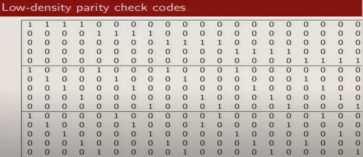
n = 20, j = 3, k = 4. where, n is codeword length, j is column weight, k is row weight.

parity check set tree is a graphical reprsentation of parity check sets in a tree like structure.

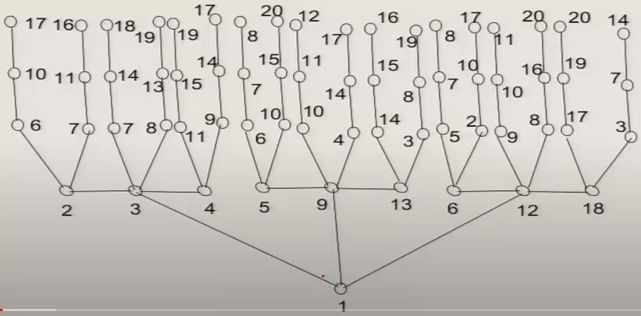
Here in the above figure, node 1 or bit no 1 is participating in three parity check equations. parity check sets: 1 => 1,2,3,4; 2 => 5,6,7,8; 3 => 9,10,11,12; 4 => 13,14,15,16; 5 => 17,18,19,20... And so on... Up to 15 party check nodes.

System model

Let, a LDPC code C(n,k) over GF(q) of length n and dimension k. the information or message symbols u=[u0, u1,…, uk-1] is encoded by LDPC encoder. Then formed codeword C= [c0, c1,…,cn-1]. Where, u(k) & c(n) both belongs to GF(q). then codeword C is mapped to constellation. When a signal is transmitted through additive white Gaussian noise channel then, y= s+n; n is complex Gaussian noise with zero mean and N0/2 per dimension.

we know in case of wireless transmission signal reach to receiver in multipath. so channel matrix are highly correlated. In case of 5G communication it uses millimetre wave band (ranges from 30-300GHz), so few strong multipath reaches to receiver and rest are to weak to detect. So channel matrix becomes sparse. In case of OFDM system it contains subcarriers. Where a vector x=[x0, x1,….,xn-1]T, where xi is a symbol transmitted in the ith subcarrier of OFDM channel.

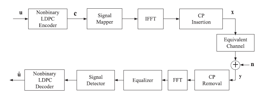
Fig : Nonbinary LDPC-coded OFDM system over multipath fading channels.

Summary

LDPC codes are sparse in nature. Here number of ‘1’ is less compared with number of ‘0’s. it is constructed from sparse tanner graph. It gives excellence performance in modern days wireless network. With comparison with other coding techniques it gives better spectral efficiency for high code rates.

References

[1] Feng, D., Xu, H., Zhang, Q., Li, Q., Qu, Y. and Bai, B. Nonbinary LDPC-Coded Modulation System in High-Speed Mobile Communications. IEEE Access, 6, pp.50994-51001, 2018.

[2] El Hassani, S., Hamon, M.H. and Pénard, P. A comparison study of binary and non-binary LDPC codes decoding. In SoftCOM 2010, 18th International Conference on Software, Telecommunications and Computer Networks (pp. 355-359). IEEE, September, 2010.

[3] Zhan, M., Pang, Z., Dzung, D. and Xiao, M. Channel coding for high performance wireless control in critical applications: Survey and analysis. IEEE Access, 6, pp.29648-29664, 2018.

[4] Davey, M.C. and MacKay, D.J. Low density parity check codes over GF (q). In 1998 Information Theory Workshop (Cat. No. 98EX131) (pp. 70-71). IEEE, June, 1998.

[5] Zhou, B., Zhang, L., Kang, J., Huang, Q., Lin, S. and Abdel-Ghaffar, K. Array dispersions of matrices and constructions of quasi-cyclic LDPC codes over non-binary fields. In 2008 IEEE International Symposium on Information Theory (pp. 1158-1162). IEEE, July, 2008.

[6] Peng, R. and Chen, R.R. WLC45-2: Application of nonbinary LDPC codes for communication over fading channels using higher order modulations. In IEEE Globecom 2006 (pp. 1-5). IEEE, November, 2006.

📚 Further Reading

• 🔗 Source Coding: Huffman Encoding and Decoding
• 🔗 Reed-Solomon Coding and Decoding
• 🔗 MS to BS Communication in LTE/5G: Sync and Pilot Allocation

Information and Coding Theory Main Page >
5G Technology Main Page >

People Also Ask (LDPC FAQ)

Why is it called "Low Density"?

Because the number of 1s in the parity-check matrix H is very small compared to the number of 0s. This sparsity makes decoding computationally feasible.

Does LDPC perform better than Turbo codes?

At very high data rates (5G speeds), LDPC is superior because it allows for massive parallel processing, whereas Turbo codes have a high-latency serial bottleneck.

LDPC vs. Turbo vs. Polar Codes

In 5G NR, LDPC was selected for data channels while Polar codes are used for control channels. Here is how they compare:

Feature	LDPC Codes	Turbo Codes	Polar Codes
Standard	5G Data (eMBB)	4G LTE Data	5G Control Channels
Latency	Ultra-Low (Parallel)	High (Serial)	Moderate
Decoding	Belief Propagation	MAP Algorithm	Successive Cancellation
Throughput	Very High (>20 Gbps)	Limited	High

Turbo Code in MATLAB (Click here)

The Future: AI & 6G LDPC

As we move toward 6G Technology, LDPC codes are evolving to meet the demands of Terahertz (THz) communication and AI-native networks:

Neural LDPC Decoders

Deep Learning models are replacing traditional Belief Propagation. Neural networks learn the "weights" of the Tanner graph to decode signals with fewer iterations and higher accuracy in non-Gaussian noise.

Quantum LDPC Codes

Researchers are adapting LDPC principles for Quantum Error Correction (QEC). CSS-type LDPC codes are being studied to protect quantum qubits from decoherence.