
MATLAB Code for Constellation Diagrams of ASK, FSK, and PSK


MATLAB Script

% The code is developed by SalimWireless.Com

clc;

clear;

close all;


% Parameters

numSymbols = 1000; % Number of symbols to simulate

symbolIndices = randi([0 1], numSymbols, 1); % Random binary symbols (0 or 1)


% ASK Modulation (BASK)

askAmplitude = [0, 1]; % Amplitudes for binary ASK

askSymbols = askAmplitude(symbolIndices + 1); % Modulated BASK symbols


% FSK Modulation (Modified BFSK with 90-degree offset)

fs = 100; % Sampling frequency

symbolDuration = 1; % Symbol duration in seconds

t = linspace(0, symbolDuration, fs*symbolDuration);

fBase = 1; % Base frequency

frequencies = [fBase, fBase]; % Same frequency for both


% Generate FSK symbols with 90° phase offset

fskSymbols = arrayfun(@(idx) ...

    cos(2*pi*frequencies(1)*t) * (1-idx) + ...

    1j * cos(2*pi*frequencies(2)*t) * idx, ...

    symbolIndices, 'UniformOutput', false);


% Extract last points (constellation points)

fskConstellation = cellfun(@(x) x(end), fskSymbols);


% PSK Modulation (BPSK)

pskSymbols = exp(1j * pi * symbolIndices); % Binary PSK symbols in complex plane


% Plotting

figure;


% ASK Constellation Diagram

subplot(1, 3, 1);

scatter(real(askSymbols), zeros(size(askSymbols)), 'filled');

grid on;

title('Binary ASK (BASK) Constellation');

xlabel('In-phase');

ylabel('Quadrature');

axis([-1.5 1.5 -1.5 1.5]);


% FSK Constellation Diagram

subplot(1, 3, 2);

scatter(real(fskConstellation), imag(fskConstellation), 'filled');

grid on;

title('Binary FSK (BFSK) Constellation with 90° Offset');

xlabel('In-phase');

ylabel('Quadrature');

axis([-1.5 1.5 -1.5 1.5]);


% PSK Constellation Diagram

subplot(1, 3, 3);

scatter(real(pskSymbols), imag(pskSymbols), 'filled');

grid on;

title('Binary PSK (BPSK) Constellation');

xlabel('In-phase');

ylabel('Quadrature');

axis([-1.5 1.5 -1.5 1.5]);

web('https://www.salimwireless.com/search?q=ask%20fsk%20psk', '-browser');

Output


Copy the MATLAB Code above from here


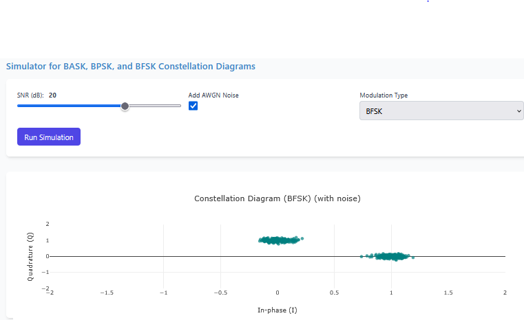
Online Simulators for Constellation Diagrams of ASK, FSK, and PSK


Explore Signal Processing Simulations


Further Reading


Contact Us

Name

Email *

Message *

Popular Posts

MIMO Channel Matrix | Rank and Condition Number

MIMO / Massive MIMO MIMO Channel Matrix | Rank and Condition...   The channel matrix in wireless communication is a matrix that describes the impact of the channel on the transmitted signal. The channel matrix can be used to model the effects of the atmospheric or underwater environment on the signal, such as the absorption, reflection or scattering of the signal by surrounding objects. When addressing multi-antenna communication, the term "channel matrix" is used. Let's assume that only one TX and one RX are in communication and there's no surrounding object. Here, in our case, we can apply the proper threshold condition to a received signal and get the original transmitted signal at the RX side. However, in real-world situations, we see signal path blockage, reflections, etc.,  (NLOS paths [↗]) more frequently. The obstruction is typically caused by building walls, etc. Multi-antenna communication was introduced to address this issue. It makes diversity app...

BER vs SNR for M-ary QAM, M-ary PSK, QPSK, BPSK, ...(MATLAB Code + Simulator)

Bit Error Rate (BER) & SNR Guide Analyze communication system performance with our interactive simulators and MATLAB tools. 📘 Theory 🧮 Simulators 💻 MATLAB Code 📚 Resources BER Definition SNR Formula BER Calculator MATLAB Comparison 📂 Explore M-ary QAM, PSK, and QPSK Topics ▼ 🧮 Constellation Simulator: M-ary QAM 🧮 Constellation Simulator: M-ary PSK 🧮 BER calculation for ASK, FSK, and PSK 🧮 Approaches to BER vs SNR Calculation What is Bit Error Rate (BER)? The BER indicates how many corrupted bits are received compared to the total number of bits sent. It is the primary figur...

UGC NET Electronic Science Previous Year Question Papers with Solutions

Home / Engineering & Other Exams / UGC NET 2026 PYQ ⬇️ Download Papers and Solutions 📋 Exam Pattern 💡 Preparation Tips ❓ FAQs 📊 Exam Highlights: Electronic Science (88) Feature Details Junior Research Fellowship (JRF) ₹37,000 + HRA per month Eligibility M.Sc/M.Tech in Electronics (55%) Validity of Certificate JRF (3 Years) | Lectureship (Lifetime) 📥 Download UGC NET Electronics PDFs Complete collection of previous year question papers, answer keys and explanations for Subject Code 88. Start Downloading 📂 View All Question Papers June 2025 - Question Paper Download PDF June 2025 - Solved Paper + Explanation ...

How to Mount Google Drive in Google Colab

How to Mount Google Drive in Google Colab Google Colab provides temporary storage during a session. Any files stored in the /content directory will be deleted when the runtime disconnects. To store datasets, trained models, and results permanently, it is recommended to mount your Google Drive in Colab. Mounting Google Drive allows your notebook to access files directly from your Drive and save outputs there so they remain available even after the Colab session ends. Step 1: Import the Drive Module First import the Google Colab drive module. from google.colab import drive Step 2: Mount Google Drive Run the following command to mount your Google Drive. from google.colab import drive drive.mount('/content/drive') After running the command: A link will appear in the output. Click the link and log in to your Google account. Copy the authentication code provided. Paste the code back into the notebook. Or, a Google authentication page will a...

Constellation Diagrams of ASK, PSK, and FSK (with MATLAB Code + Simulator)

Constellation Diagrams: ASK, FSK, and PSK Comprehensive guide to signal space representation, including interactive simulators and MATLAB implementations. 📘 Overview 🧮 Simulator ⚖️ Theory 📈 Q-function 📚 Resources BASK Modulation Transmits one of two signals: 0 or $\sqrt{E_b}$, representing binary 0 and 1. Simple but sensitive to noise. BFSK Modulation Transmits one of two signals: $\sqrt{E_b}$ on the Y-axis or $\sqrt{E_b}$ on the X-axis. These are orthogonal signals. BPSK Modulation Transmits $+\sqrt{E_b}$ or $-\sqrt{E_b}$ (antipodal signaling). Most efficient binary scheme. ...

Wiener Filter in MATLAB

  MATLAB Code  % Wiener Filter Based on Wiener-Hopf Equation % This script demonstrates how to apply the Wiener filter to recover % a reference signal from a noisy signal using the Wiener-Hopf equation. % The filter minimizes the mean squared error between the noisy signal and the reference signal. clear; close all; clc; % Signal Parameters fs = 4000; % Sampling frequency (Hz) T = 1; % Total recording time (seconds) L = T * fs; % Signal length (samples) tt = (0:L-1) / fs; % Time vector ff = (0:L-1) * fs / L; % Frequency vector % Generate Reference Signal (a sinusoid) y = sin(2 * pi * 120 * tt); % Reference sinusoidal signal y = y(:); % Ensure column vector % Create Noisy Signal by Adding Gaussian Noise x = 0.50 * randn(L, 1) + y; % Noisy signal x = x(:); % Ensure column vector % Define Filter Order (Number of Coefficients) N = 200; % Apply Wiener Filter using custom function [xest, b, MSE] = wienerFilt(x, y, N); % Plot Results figure; subplot(411); plot(tt, x, 'k'), hold on, p...

Overmodulation & Distortion in AM

Overmodulation in AM and How It Causes Distortion 1. AM Signal Equation s(t) = A c [1 + μ m(t)] cos(2Ï€ f c t) A c = carrier amplitude m(t) = normalized modulating signal (|m(t)| ≤ 1) μ = modulation index 2. Modulation Index μ = A m / A c - Normal AM: 0 < μ ≤ 1 → no distortion - Overmodulation: μ > 1 → distortion occurs 3. Envelope and Overmodulation A(t) = A c [1 + μ m(t)] - For undistorted AM: 1 + μ m(t) ≥ 0 at all times - If μ > 1: 1 + μ m(t) < 0 at negative peaks → carrier flips Example: Let m(t) = cos(2Ï€ f m t), A c = 1 V, μ = 1.2 Minimum envelope: A min = A c [1 - 1.2] = -0.2 V Negative amplitude → envelope crosses zero → 180° phase flip 4. Mathematical Consequence -A c cos(θ) = A c cos(θ + Ï€) This phase reversal is what causes distortion in the demodulated signal. 5. Instantaneous AM Signal s...

Phase Modulation (PM) & Demodulation

Advanced Analysis of Phase Modulation Phase Modulation (PM): Theoretical Foundations and Spectral Dynamics 1. Analytical Characterization Phase Modulation (PM) is a subset of Angle Modulation , where the information residing in the message signal \( m(t) \) is mapped linearly onto the instantaneous phase of a high-frequency carrier. Unlike Amplitude Modulation (AM), PM is a non-linear modulation process, resulting in an expansion of the signal bandwidth into an infinite dimensional Hilbert space. \[ S_{PM}(t) = A_c \cos\left[ 2\pi f_c t + \phi(t) \right] = A_c \cos\left[ 2\pi f_c t + K_p m(t) \right] \] The instantaneous frequency \( f_i(t) \) is defined as the time derivative of the total angle: \[ f_i(t) = \frac{1}{2\pi} \frac{d\theta_i(t)}{dt} = f_c + \frac{K_p}{2\pi} \frac{dm(t)}{dt} \] ...