Fourier Transform of some common analog signals

• Fourier Transform of a delta function

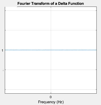
If x(t) = \( \delta(t) \), then Fourier transform,

X(\( \omega \)) = \( \int_{-\infty}^{\infty} \delta(t)e^{-j\omega t} dt \)

= \( \int_{-\epsilon}^{\epsilon} \delta(t)e^{-j\omega t} dt \)

= \( \int_{-\epsilon}^{\epsilon} \delta(t)e^{-j\omega 0} dt \)

= 1

Thus, the Fourier transform of a delta/impulse is a constant equal to 1, independent of frequency. Remember that derivation used the shifting property of the impulse to eliminate the integral.

 

 

 

• Fourier transform of a unit step function

 

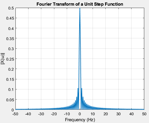
\( \gamma(t) \) = 0 for t < 0

                                                            = 1 for t \( \ge \) 1

We know that a unit-step function is an integration of a delta function. So for a unit step function,

\( \gamma(t) \) = \( \int \delta(t) dt \)

So, X(\( \omega \)) = \( \frac{1}{j\omega} F(\delta(t)) + \pi F(\delta(t))\delta(\omega) \)

[See the property of integration above]

           = \( \frac{1}{j\omega} + \pi\delta(\omega) \)       [as F(\( \delta(t) \)) = 1]

When a function (i.e., x(t)) is not an energy function and hence the Fourier transform of [\( \int x(t) dt \)] includes an impulse function.

 

 

 

• Fourier Transform of a rectangular / unit pulse function

A pulse function can be represented as,

x(t)=Π(t) = \( \gamma(t + \frac{1}{2}) - \gamma(t - \frac{1}{2}) \)

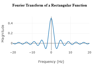
For a function rect(t) = Π(t) = 1 for |t| \( \le \frac{1}{2} \)

                                             = 0 otherwise

Given that

x(t) = Π(t)

Hence from the definition of the Fourier transform we have

F (Π(t)) = X(\( \omega \)) = \( \int_{-\infty}^{\infty} \Pi(t)e^{-j\omega t} dt \)

                           = \( \int_{-1/2}^{1/2} e^{-j\omega t} dt \)      [as Π(t) = 1 for |t| \( \le \frac{1}{2} \)]

                            = [(e ^–jωt)/-jω]_-1/2^1/2

                                           = [e ^–jω/2 - e ^jω/2] / -jω

                            = [e ^jω/2 - e ^-jω/2] / jω

                            = 2/ω . {[e ^jω/2 - e ^-jω/2] / 2j}

                            = 2/ω . sin(ω/2)

                            = {sin(ω/2) / (ω/2)}

                           = {sin(\( \pi \)(ω/2\( \pi \))) / (\( \pi \)(ω/2\( \pi \)))}

                            = sinc(ω/2\( \pi \))

 

For the above case, the rectangular function has a pulse width value of 1 over the interval of [-½, ½]; 0 otherwise.

Now we’ll discuss a rectangular pulse that has a width of T

Then,    rect(t/T) = Π(t/T) = 1 for |t| \( \le \) T/2

                                             = 0 otherwise

Given that

x(t/T) = Π(t/T)

Hence from the definition of the Fourier transform we have

F (Π(t/T)) = \( \int_{-\infty}^{\infty} \Pi(t/T)e^{-j\omega t} dt \)

                           = \( \int_{-T/2}^{T/2} e^{-j\omega t} dt \)      [as Π(t/T) = 1 for |t| \( \le \) T/2]

                            = [(e ^–jωt)/-jω]_-T/2^T/2

                                           = [e ^–jωT/2 - e ^jωT/2] / -jω

                            = [e ^jωT/2 - e ^-jωT/2] / jω

                            = 2/ω . {[e ^jωT/2 - e ^-jωT/2] / 2j}

                            = 2/ω . sin(ω(T/2))

                            = {sin(ω(T/2)) / (ω/2)}

                            = {sin(\( \pi \)ωT/2\( \pi \))) / (\( \pi \)ω/2\( \pi \))}

                            = {sin(\( \pi \)ωT/2\( \pi \))) / (\( \pi \)ωT/2\( \pi \))}.T

                            = T. sinc(ωT/2\( \pi \))

 

 

 

 

• Fourier Transform of a unit triangle pulse

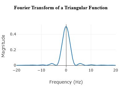
A unit triangle pulse is simply the convolution of a unit pulse function with itself.

Here, Λ(t) = Π(t) * Π(t)               

[Π(t) is a unit pulse function & ‘*’ denotes convolution]

So, Λ(\( \omega \)) = sinc(ω/2\( \pi \)) . sinc(ω/2\( \pi \)) = sinc²(ω/2\( \pi \))

 

 

 

• Fourier Transform of a Sawtooth function

s(t) = 0, for t < 0 and t > 1

                                                  = t, for 0 \( \le \) t \( \le \) 1

We can represent sawtooth as the integral of shifted unit pulse function (to give the ramp) and a negative impulse (delayed by one second) to give the discontinuity at the end of the ramp

 

s(t) = \( \int_{-\infty}^{t} \Pi(\tau)d\tau - \int_{-\infty}^{t} \delta(\tau-1)d\tau = \int_{-\infty}^{t} y(\tau)d\tau \)

y(t) = \( \Pi(t) - \delta(t-1) \)

Now, we’ve to find the Fourier transform of y(t),

Y(\( \omega \)) = sinc(ω/2\( \pi \))e^-jω/2 - e^-jω

We can now apply integral property with Y(0) = 0, to find S(\( \omega \))

S(\( \omega \)) = F(\( \int_{-\infty}^{t} y(\tau)d\tau \)) = Y(\( \omega \))/jω - \( \pi \)Y(0)\( \delta \)(0) = Y(\( \omega \))/jω

= {(sinc(ω/2\( \pi \))e^-jω/2 - e^-jω) / jω}

= {((sin(π . ω/2\( \pi \)) / (π . ω/2\( \pi \)))e^-jω/2 - e^-jω) / jω}

=  (((sin(π . ω/2\( \pi \)) / (π . ω/2\( \pi \)))e^-jω/2) / jω) – (e^-jω / jω)

= (2(sin(ω/2)e^-jω/2) / jω²) – (je^-jω / j²ω)

= (2((e^jω/2 - e^-jω/2) / 2j)e^-jω/2) / jω²) + (je^-jω / ω)     [as j² = -1]

= (((e^jω/2 - e^-jω/2)e^-jω/2) / j²ω²) + (je^-jω / ω)

= (((e^-jω/2 - e^jω/2)e^-jω/2) / ω²) + (je^-jω / ω)

= (((e^-jω/2 - e^jω/2)e^-jω/2) / ω²) + (je^-jω / ω)

= ((((e^-jω/2 - e^jω/2)e^-jω/2) + jωe^-jω) / ω²)

= ((e^-jω - 1 + jωe^-jω) / ω²)

= ((e^-jω(1+jω) - 1) / ω²

Further Reading

1.