Adaptive Channel Estimation for Millimeter wave 5G

Adaptive Channel Estimation

7.1. Introduction

Channel estimation is to acquire site specific channel model of a particular environment. Millimetre wave cannot travel much distance in atmosphere due to its severe pathloss and high refraction properties. It also experiences high penetration loss. So, we need to equip MIMO system to avail beamforming. And it is also needed to deploy large antenna arrays in MIMO system to form narrower and stronger beam to fulfil the link margin gain at receiver side.

So, we need to train the beam to find the best beamforming vector at transmitter side and best combing vector pair at receiver side to maximize the signal to noise ratio. The beam training can be realized by analog beamformer but the limitation of analog beamforming is that only one data stream with same amplitude and different phases is possible. That cannot provide high data rates as required. That’s why we need to focus on MIMO hybrid architecture. In that architecture analog beam steering is realized by large antenna arrays and baseband precoding is realized by low dimensional digital precoder. It also helps us to maintain low overhead in network.

Especially, for vehicular communication channel varies fast, so, channel estimation plays a crucial role to find the best communicating beam from BS to find the best signal to noise ratio from beam steering.

7.2. System Model:

In MIMO channel estimation process, firstly we train the beam using beam steering method to pick the best beam from Tx and Rx side both. There is only one RF chain available in analog precoder with can enable single data stream between transmitter and receiver. So, we further go for hybrid architecture with equips lower dimensional baseband precoder which enables multiple simultaneous data stream and cancel interference between them as shown in figure 7.1.

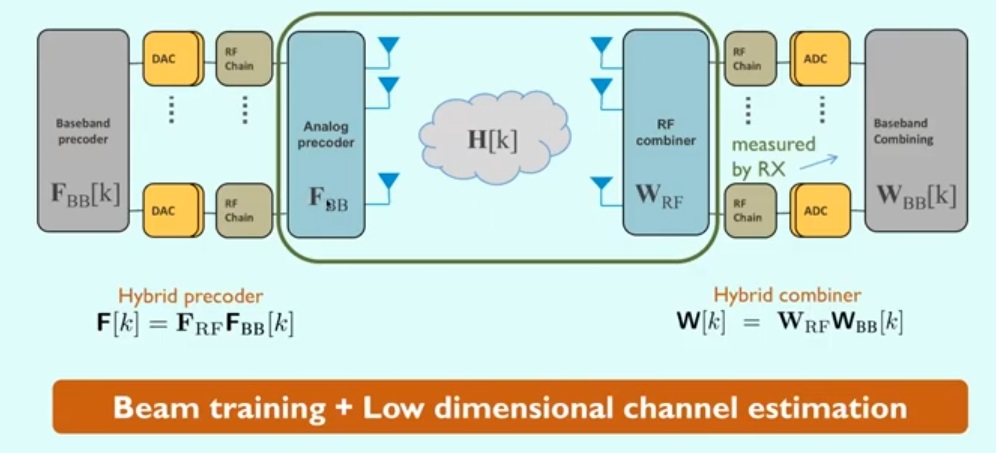
Fig 7.1: Architecture of transceiver at Tx & Rx both which contains RF chains and baseband beamformers

On the other hand, hybrid precoder is used for low overhead in network because it uses relatively lesser RF chain as compare to digital optimal precoder without compromising much in performance.

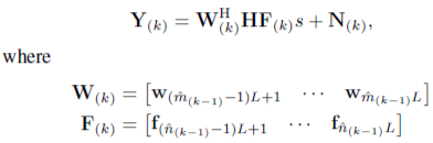
Here I will discuss communication between a BS (base station) and vehicles for mm Wave communication channel. Both N_BS and N_v have linear arrays (ULAs), with half-wavelength spaced antenna elements in a compact area uniformly. Let assume, f_n is the beamforming vector at BS side. BS need to transmit a symbol, s, such that |s|² = 1. On the other hand, vehicle assigns a unit-norm measurement vector w_m. Now, the signal received at MS (user) side is written by

…………………………………………..(Appendix B)

Here in above equation BS and MS both enable beam steering. At a moment they find the best beam pairs to enable communication. Here ‘m’ indicates best beamforming vector from BS and ‘n’ from receiver side.

In the above figure 7.1, BS employs baseband precoder, F_BB of size N_RF X N_S which is followed by RF precoder, F_RF of size N_BS X N_RF. BS can communicate to MS thru N_S data streams simultaneously and similarly it is applicable to MS side, where N_S ≤ N_RF ≤N_BS and, N_S ≤N_RF≤N_MS. Number of maximum possible simultaneous data streams between Tx and Rx is always less than or equal to number of RF chain.

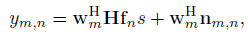
If F_T= F_RF F_BB is the combined then BS precoding matrix is of size N_BS X N_S, then transmitted signal is denoted by,

……………………………………………………………………….(7.1)

We know in case of mmWave channel estimation most of MPCs are so weak that makes mmWave channel matrix sparse. Only few MPCs are strong to avail communication between Tx and Rx. Let assume, the numbers of energy rich limited MPCs are L. Now, L MPCs contain AOA & AOD, and corresponding gain of each path. It is now essential to build the BS and MS training precoders and combiners in order to reduce the training overhead.

We’ll take advantage of the mmWave channel’s low scattering properties. Which indicates low rank property of the millimetre wave channel matrix or estimation problem as a sparse problem. It is shown here how adaptive compressed sensing (CS) works on certain objectives to find the training precoders and combiners for low overhead mmWave band communication. A novel hierarchical multi resolution codebook based on the hybrid analog/digital interface architecture is used to train beamforming vectors.

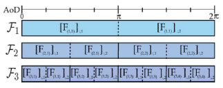
Fig 7.2: With beamforming vectors in each subset, architecture of a multi-resolution codebook with total beamforming vector N=8 and, total stage, K=2.

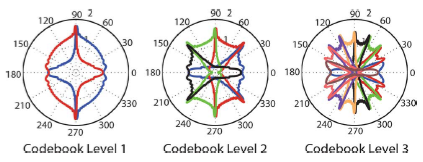
Fig 7.3: The beampatterns for the resulting beamforming vectors are shown in the first three codebook layers of an example hierarchical codebook.

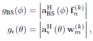
In the above figure 7.2, let assume we want to cover the transmitted signal from BS in all directions in 0 to 360 degree azimuth angle range around the nearby area of BS. Then we divide the azimuth angle range of transmission in subparts, for example we divide it into two parts, and assign beamforming vector to each part, where one beamforming vector is supposed to cover 0 to 180 degree range and another for 180 to 360 degree range and it is only for the 1^st stage. Then in second stage each azimuth angle range is further subdivided into different parts (shown in figure 7.4) and so on, only to find best beamformer and combiner pair to maximize the SNR.

Algorithm 2: Adaptive Estimation Algorithm for Single-Path mmWave Channels

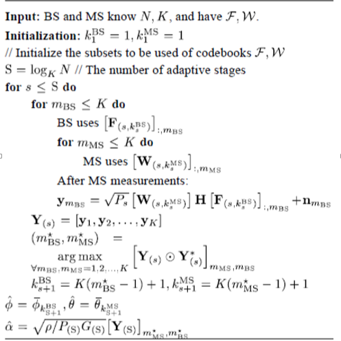
Let assume for ‘P’ number of antenna elements in Tx and ‘Q’ number of antenna element in Rx, so there will be total P X Q possible paths between BS and MS. But due to high pathloss and poor scattering nature, only few stronger MPCs reach up to receiver. Here number of detectable strong paths or MPCs is ‘N’. The BS in the above algorithm uses the K training precoding vectors at the 1st level of the multi-resolution codebook, F, at the initial step. Similarly, the MS uses the measurement vectors of the first stage of W to combine the beamforming vectors from transmitter. Now at second stage each slot of previous stage is divided into K slots and we assign beamforming vector accordingly. At the final stage the total number of beamforming vector will be K^S which is equal to total number of stronger MPCs or path, N. In adaptive estimation process we apply beam steering at different stages at find the best path with higher SNR (Alkhateeb, 2014).

7.3. Channel Estimation for Vehicular communication

The most promising technology for enabling ultra-fast and high-data-rate exchanges is mm wave communication. In case of vehicular communication BS can be placed in a particular place along road-side, or in simple word previously known location of road or infrastructure can improve initial access of communication. Millimeter wave connectivity has the advantage of supporting multi-Gbps throughput, but it suffers from substantial pathloss. On the other hand, as mm Wave wavelength lies between 1-10 millimetres so enable packing many antenna elements in a compact area.

Let assume, there is maximum L different beamforming and combining or measurement vectors is possible in different time slots at last stage (say, k^th stage) of adaptive channel estimation process. So, there is total of L X L measurements among which we have to find which beamforming and combining or measurement vector pair has higher gain at receiver side. Now, arranging in matrix form, we can write

……………………………………………………………………..(7.2)

where W = [w1,…,wL], and F = [f1,…,fL]

N ~ Noise at different time slot with zero mean and variance σ² , such that N ~ CN(0,σ²I)

Noise N are statistically independent for different time slots.

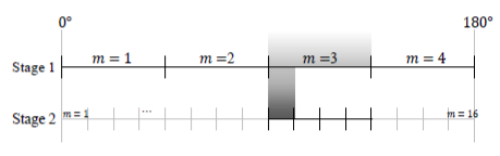
Fig 7.4: illustration of Adaptive channel estimation, where first stage contain ‘m’ number of beamforming vector at different time slot; then at stage 2, each previous time slot divided into 4 slots where each slot represents a angular range of a beamforming vector.

Here in figure, the coverage area in azimuth angular range is subdivided into four subranges and assigned a beam beamforming vector for each subrange or slot, similarly as mentioned for figure 7.3. & 7.4 above. In this adaptive channel estimation process required codebook for beamforming and measurement vector at Tx and Rx, respectively, are pre-computed if it is location aided. In this estimation process it is done in multiple stages. Our goal is to find best beamforming and measuring vector pair. At stage ‘k’ for received signal Y_(k) is denoted as,

……………………………..(7.3)

At the beginning, at first stage we assume that suitable AOD and AOA for communication lies between 0 to 180⁰ range. And four beamforming vectors cover the whole angular range by applying corresponding beamwidth as shown in figure 11. At the next stage (stage 2) AOD and AOA range for a beam forming vector is further divided into four slots. In the above equations ^m(k-1) and ^n(k-1) subscripts denotes corresponding beamforming and combining vectors at stage k-1 and so forth. The Tx and Rx sound the channel in numerous AOD and AOA ranges corresponding to various stages in this operation, and the strongest SNR achieved is chosen. The previous ranges are divided into L sub-ranges in the next level. To achieve desired RSSI we apply the next stages in this channel estimation process. If 1^st stage consists of L number of beamforming vectors then at stage k it will contain L^k independent slots. Here, it is now necessary that beamforming and combining or measurement vector will always choose from final stage k, it can be chosen from previous stages if we achieve stronger SNR at receiver side. Now, angle of arrival and departure (AOA & AOD) vector dependent gain can be denoted by,

……………………………………………………………….(7.10)

Let assume, at stage k, the range of the m-th weight vector is R_m^(k) at the Tx or Rx, where the final stage k contains L^k disjoint sub-ranges which covers the AOA or AOD range from 0⁰ to 180⁰ [0, π] . The mathematical expression for R_m^(k) is given by,

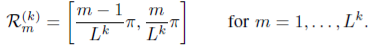……………………………….(7.4)

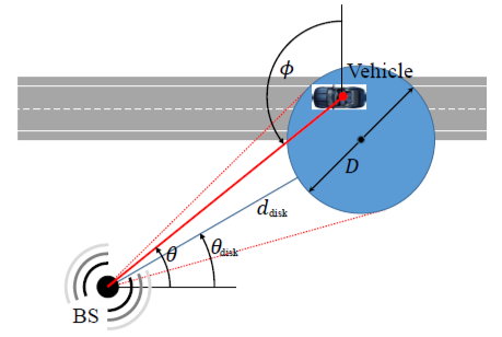
Fig 7.5: Here disc indicates priory known location information of the vehicle. Angle of departure (AOD) from BS and angle of arrival (AOA) at vehical side, which are expected to be priory known, represented as, u_θ = [θ_disk - arcsin( D/2d_disk), θ_disk + arcsin( D/2d_disk)] and u_φ = [π - θ_disk - arcsin( D/2d_disk), π -θ_disk +arcsin( D/2d_disk)] , respectively. Where, –π/2 ≤ arcsin(x) ≤ π/2 (Garcia, 2016).

By the way, channel estimation parameters totally depends on chosen number of total stages, how many beamforming vectors will be assigned at 1^st stage, and codebooks at the Tx and Rx side (Garcia, 2016).

7.4. Mm wave channel estimation in the Presence of location Information:

It is assumed that the vehicle is located in the blue disk shown in figure 12 which has radius of D. The distance from BS to the centre of the disc is d_disk where angle of departure (AOD) from BS to the centre of disk is given by, θ_disk. From the available location information, further we convert it to corresponding AOD/AOA by using basic trigonometric ratios. It has been said before that adaptive channel estimation method is multi-level process, so, which AOD/AOA range do not satisfy the link margin at receiver, is cancelled. Then we proceed to the next stage of channel estimation. Similarly, pathloss due to particular AOD/AOA can be calculated from the location information.

In the above figure 12, the priory known angle of departure (AOD) is indicated as, θ belongs to set u _θ and angle of arrival φ belongs to set u _φ ; such that sets u _φ , u _θ lies between [0, π) . Suppose, the sequences of beamforming and measurement vectors are m₍₁₎,…,m_(K) and n₍₁₎,…,n_(K), respectively, where the indices indicates the stage. If P(m_(K),n_(K)) denotes the probability of beamforming and measuring vector pairs at stage k, then,

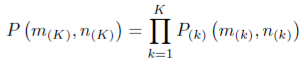…………………………………………..(7.5)

All stages in adaptive channel estimation process is independent where individual stages happen at individual time intervals. We choose a beamforming and measuring vector pair which contributes a stronger RSSI at receiver at a particular stage. The indicator for m^th beamforming vector n^th measurement weight vectors, where each slot consist of L number of beamforming vector. The SNR value for a particular stage of adaptive channel estimation is defined as

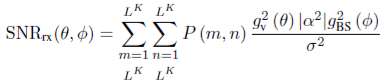……………………………..(7.6)

Where k= number of stage; α = channel gain; g_v² = Rx side antenna gain; g_BS² = Tx side antenna gain; P(m, n) is probability of m^th beamformer vector and n^th combiner vector for a particular stage.