Beamforming Techniques for Millimeter wave 5G

Beamforming Techniques

6.1. Introduction

Beamforming is a useful strategy to focus a wireless signal towards a specific direction i.e, towards the receiver to maximize the gain rather than having signal spread in all direction like omni-directional antennas. Standard analog beamforming for mm wave communication is generally contains only one RF chain and phase shifters (PSs) to send in multiple phases, which imposes constant amplitude restrictions on the analog beamformer architecture. Analog beamforming is easier to apply to hardware but it has a substantial performance loss. At low frequencies, on the other hand, digital precoding will control both the amplitude and phase of the signal. It removes interferences and achieves the best possible outcomes. For each antenna element, however, digital precoding necessitates a separate baseband and RF chain. Currently, it is both costly and energy-intensive. If hundreds or thousands of antennas are used in millimeter wave large MIMO systems, the resulting huge amount of RF chains would be prohibitively costly and energy-intensive. For example, a mm-wave RF chain's power consumption (including digital-to-analog converters and vice versa, up-converters, and so on) is about 250 Milliwatt, and RF chains will consume a total of 8 Watt in a massive MIMO device with 32 antennas for mm-wave communication. Hybrid precoding, in particular, splits the best digital precoder into two stages. Firstly, digital precoder with small number of RF chain is implemented to cancel interferences. After that, an analogue beamformer with a large number of analogue phase shifters is used with one RF chain. It improves the gain of the antenna array. As a result, hybrid precoding will greatly reduce the amount of RF chains required. Because of the cautious architecture, there is no apparent performance loss, making it a promising precoding method for millimetre wave large MIMO systems (Mumtaz, 2016).

6.2. Digital Beamforming:

For cancelling interference between multiple users, in MIMO systems, digital precoding is a popular technology. To cancel interferences in advance, it monitors the phases and amplitudes both of initial signals. Single-user precoding and multiuser precoding are the two primary forms of digital precoding.

6.2.1. Digital Beamforming for Single-User scenario:

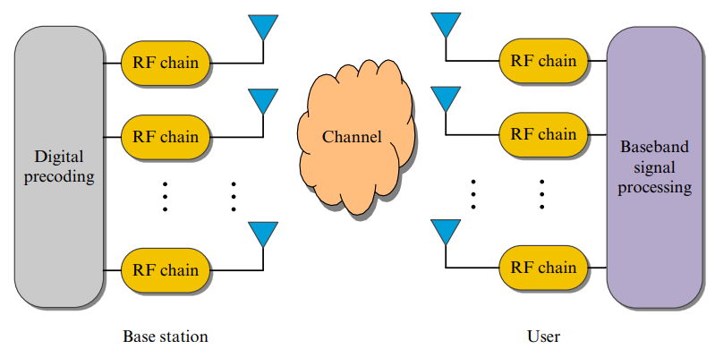
Fig 6.1: configuration of single-user digital precoder for millimetre Wave massive MIMO system (Mumtaz, 2016).

Here in fig. 6.1, BS uses N_t antennas and receiver employs N_r antennas. Transmitter can transmit at maximum N_r data streams to receiver simultaneously, where N_r < N_t. As a result, the number of simultaneous data streams transmitted is equal to the number of antennas on the receiver. Using its N_t RF chains, BS implements a N_t X N_r digital precoder D. Each antenna elements requires its own RF chain.

The received signal vector y at receiver side,

y= √ρHDs + n

Here, ρ = average received power

H =channel matrix ( N_r X N_t)

n = additive white Gaussian noise vector

(Appendix B)

6.2.2. Digital Beamforming for Multi-User scenario:

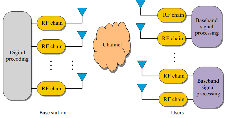
Fig 6.2: Configuration of multi-user digital precoder for millimetre Wave massive MIMO systems (Mumtaz, 2016)

Here in above figure 6.2, BS uses N_BS antennas and N_BS^RF chains for communication with U mobile stations (MSs) simultaneously. N_MS antennas are there in each MS. The total number of data streams for communication is equal to the number of antennas on the receiver side, N_MSU, where N_MSU ≤ N_BS. On the downlink side, the BS applies an N_BS X N_MSU digital precoder D (say). Where, D= [D₁, D₂, …, D_U], & D_u denotes the u th user, a digital precoder (size of N_BS X N_MS)

Now cancel interference at u^th user due to other users, we need to design the baseband precoder in such a way that H_uD_n for nǂ u should be zero at the u th MS. Therefore, H_uD_n =0 cancels interferences at uth MS. (Appendix B)

6.3. Analog Beamforming:

Analog beamforming sends same signal from multiple antennas with different phases using phase shifters (PSs) to maximize gain and effective SNR of antenna arrays in a particular direction.

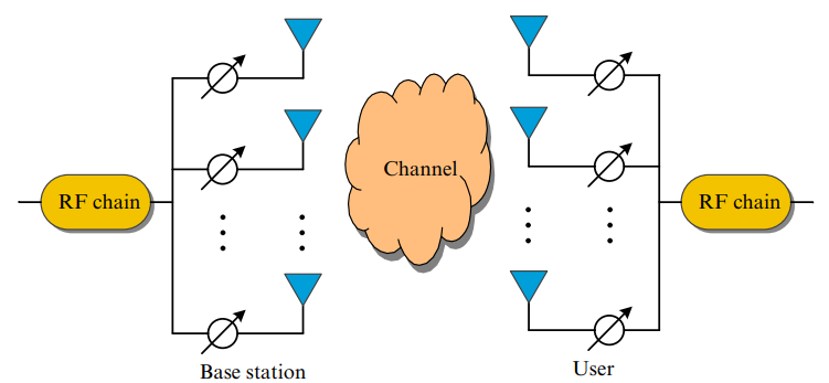
Fig 6.3: Analog beamforming configuration for single-user mm-wave

MIMO structures (Mumtaz, 2016)

6.3.1. Beam Steering:

BS transmits one data stream to a device using Nr antennas and just one RF chain using N_t antennas which is shown in figure 6.3. Let f be the analogue beamforming vector at the BS (transmitter side) of size N_t X 1 and w be the analogue combining vector at the consumer of size Nr X 1. (receiver side). The goal is to choose effective f and w pair in order to optimise the signal to noise ratio, which can be written as,

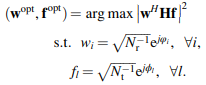…………………………………(6.1)

Beam Training:

During beam training, BS and MS both use predefined codebooks to find the right beamformer and combiner pair to maximize the channel gain. In the below figure 6.4, it is shown that firstly, BS applies beam steering at MS side while the MS enables omni-directional transmistion and similarly in next step MS applies beam steering and BS acts as omni-directional transmitter. Then best beamformer and combiner pair at BS & MS is found and they avail communication. The codebook can be outlined as follows:

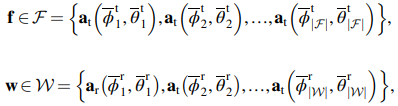…………(6.2)

The quantified azimuth (elevation) angles of departure and arrival are, respectively, ϕ^t _l (θ^t _l ) and ϕ_l^r (θ^r _l), That are assumed to cover the full ranges of angle of arrivals/departures (AoDs/AoAs) uniformly.

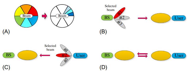
Fig 6.4: The hierarchical beam training methodology includes a multilevel codebook, a beam sweep on the BS side, a beam sweep on the user side, and a feedback procedure (Mumtaz, 2016)

6.4. Hybrid Beamforming:

We apply Hybrid beamforming to balance flexibility and cost trade-offs but still meets the needed performance parameters. It faces some drawbacks when we extend MIMO into massive MIMO in mm-wave with digital precoding and analog beamforming. To resolve this issue, digital precoding and then analog beamforming is applied. In the first stage, a small-size digital precoder is used to cancel interferences, and then a large-size analog beamformer is used to increase the antenna array gain.

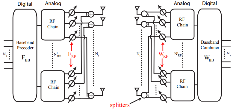
Fig 6.5: Architecture of single user system in mm-wave that uses digital baseband precoding, then implements analog beamforming using RF phase shifters (PSs) (El Ayach, 2014)

Here in above figure hybrid precoder is subdivided into analog precoder equipped with larger antenna array and relatively small baseband or digital precoder to cancel interference between simultaneous multiple data stream available in MIMO communication system between Tx & Rx due to spatial multiplexing compatibility.

The signal received by users vector y,

y = √ρHADs + n

where, H=Channel Matrix

n = additive white Gaussian noise (AWGN)

(Appendix B)

6.4.1. Spatially sparse hybrid precoding:

Each antenna element in a completely connected architecture must have its own radio frequency (RF) series. The analog phase shifter (PSs) applies the analog beamformer; all of its elements have the same amplitude but different phases. The goal is to optimise the overall throughput or sum rate R (A, D) obtained over Gaussian signalling on MMwave channels by designing (A, D).

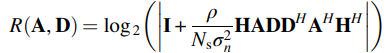..........................................(6.3)

The related sum rate optimization problem looks like this:

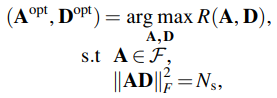……………………. (6.4)

Here, set F consists all possible analog beamformers (size of N_t X N_RF^t matrices) with constant-magnitude entries.

Now for hybrid architecture we will find singular value decomposition (SVD) of channel matrix to find the stronger eigen values and we will only allocate power accordingly to these paths to achieve low overhead in hybrid architecture (Appendix B). For example we will further divide the eigen value matrix (Σ) into two parts (Eqn 6.5) where Σ₁ is a N_s X N_s matrix; where N_s indicates rank of matrix or how many simultaneous data streams are available between BS and MS

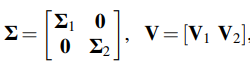………………………… (6.5)

On the other hand optimal unconstrained precoding is called fully digital precoding which is based on the singular value decomposition (SVD) of the channel matrix where we allocate power to each eigen path. Hybrid beamforming employs less number of RF chain in case of multiple-stream transmission as well as concept of OMP (orthogonal matching pursuit) is used (El Ayach, 2014).

6.5. Advantages of Hybrid Beamforming:

1. In digital beamforming, applied RF chain is equal to the number of antenna elements. Where in Hybrid beamforming only few RF chains are required for same number of antenna elements without compromising much. It also reduces cost.

2. Massive MIMO with spatial multiplexing technique enhances larger capacity. Without hybrid beamforming, digital beamforming is prone to beamforming inaccuracy , unaffordable or complex

3. As beamforming focuses high gain signal in specific direction, so, it reduces the channel coherent time. On the other hand, as hybrid beamforming uses a few RF chain unlike digital beamforming circuitry, so, it needs less power to transmit and receive data (Ahmed, 2018).

6.6. Spatially sparse Hybrid Beamforming using OMP

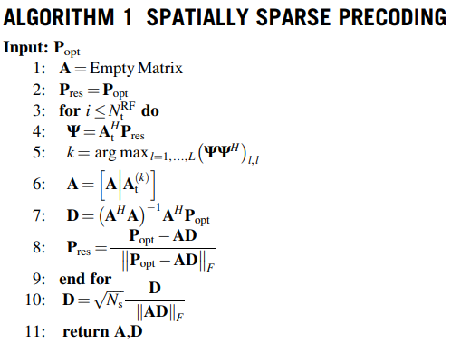
In the above algorithm, we get vector A_t(ϕ_l^t , θ_l ^t ) which is transmission array vector along with P_opt (which is basically unitary ‘V’ matrix in SVD (appendix B)) has maximal projection in step 5. A_t(ϕ_l^t , θ_l ^t ) also indicates antenna array vector at transmitter with a azimuth and elevation angle of departure. Here in Step 6, the chosen column vector A_t(ϕ_l^t , θ_l ^t ) is applied to the analogue beamformer A. Step 7 involves deciding the dominant vector as well as D's least-squares (LS) solution. ‘D’ indicates digital precoder. The chosen vector's input is then omitted in Step 8, and the method must begin detecting the column along which the Pres (Residual precoding) matrix has the highest projection before all N_t RF precoding vectors have been selected (Mumtaz, 2016).