Gauss Jacobi Method

Gauss Jacobi Method

In numerical linear algebra, the Gauss-Jacobi method (the Jacobi iteration method) is an iterative algorithm for determining the solutions of a strictly diagonally dominant system of linear equations.

Procedure

1. Choose an n X n matrix

Otherwise- Show Pop up – please select the number of rows equal to the number of Columns

2. Verify that the magnitude of the diagonal item in each row of the matrix is greater than or equal to the sum of the magnitudes of all other (non-diagonal) values in that row so that

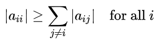
Otherwise- Show Pop up – entered matrix is not diagonally dominant

Ensure that all of the diagonal elements are non-zero as well.

a_ii ≠ 0

Otherwise- Show Pop up – all of the diagonal elements must be non-zero

3. Decompose the given matrix into a diagonal matrix D, a lower triangular matrix L, and an upper triangular matrix U:

Let’s assume, A linear system of the form ��=�Ax = b

A = $\begin{bmatrix} a11 & a12 & \cdots & a1n \\ a21 & a22 & .\ .\ . & a2n \\ \vdots & \vdots & \ddots & \vdots \\ an1 & an2 & \cdots & ann \end{bmatrix}$; D = $\begin{bmatrix} a11 & 0 & \cdots & 0 \\ 0 & a22 & .\ .\ . & 0 \\ \vdots & \vdots & \ddots & \vdots \\ 0 & 0 & \cdots & ann \end{bmatrix}$;

L + U = $\begin{bmatrix} 0 & a12 & \cdots & a1n \\ a21 & 0 & .\ .\ . & a2n \\ \vdots & \vdots & \ddots & \vdots \\ an1 & an2 & \cdots & 0 \end{bmatrix}$;

Where,

A = D + L + U

D contains only the main diagonal elements of matrix A & (L + U) = A – D

4. Consider solving a n X n (n by n) matrix then initially take a column matrix X⁽⁰⁾ of size n X 1 containing only 1s

X⁽⁰⁾ = $\begin{bmatrix} x1 \\ x2 \\ \vdots \\ xn \end{bmatrix}$, where, x₁ = x₂ = x₃ = . . . = x_n = 1

5. Then calculate,

X⁽¹⁾ = D^-1 (b – (L + U) X⁽⁰⁾)

Or, X⁽¹⁾ = D^-1 (b – (L + U) X⁽⁰⁾)

D^-1 or the inverse of a diagonal matrix is a diagonal matrix where the elements of the main diagonal are the reciprocals of the corresponding elements of the original diagonal matrix. Or,

D^-1 = $\begin{bmatrix} 1/a11 & 0 & \cdots & 0 \\ 0 & 1/a22 & .\ .\ . & 0 \\ \vdots & \vdots & \ddots & \vdots \\ 0 & 0 & \cdots & 1/ann \end{bmatrix}$;

Then check, ||AX⁽¹⁾ – b|| is small or not

If ||A X¹ – b|| is not small then go for the 2^nd iteration

X⁽²⁾ = D^-1 (b – (L + U)X⁽¹⁾)

Continue to the next iteration if the condition is still unsatisfied

Example

Use the iterative Gauss-Jacobi method to solve the problem. There are equations

2x + y = 13

5x + 7y = 11

Taking values from the aforementioned equations, we obtain,

A = $\begin{bmatrix} 2 & 1 \\ 5 & 7 \end{bmatrix}$; b = $\begin{bmatrix} 13 \\ 11 \end{bmatrix}$;

Now, D = $\begin{bmatrix} 2 & 0 \\ 0 & 7 \end{bmatrix}$; L + U = $\begin{bmatrix} 0 & 1 \\ 5 & 0 \end{bmatrix}$;

Let’s initialize, x⁽⁰⁾ =$\begin{bmatrix} 1 \\ 1 \end{bmatrix}$;

Then calculate,

1^st iteration

X⁽¹⁾ = D^-1 (b – (L + U)X⁽⁰⁾)

= -D^-1(L + U) X⁰ + D^-1b

= $- \begin{bmatrix} 1/2 & 0 \\ 0 & 1/7 \end{bmatrix}\begin{bmatrix} 0 & 1 \\ 5 & 0 \end{bmatrix}$ $\begin{bmatrix} 1 \\ 1 \end{bmatrix}$ + $\begin{bmatrix} 1/2 & 0 \\ 0 & 1/7 \end{bmatrix}\begin{bmatrix} 13 \\ 11 \end{bmatrix}$

= - $\begin{bmatrix} 0 & 1/2 \\ 5/7 & 0 \end{bmatrix}\begin{bmatrix} 1 \\ 1 \end{bmatrix}$ + $\begin{bmatrix} 13/2 \\ 11/7 \end{bmatrix}$

= $\begin{bmatrix} - 1/2 \\ - 5/7 \end{bmatrix} + \ \begin{bmatrix} 13/2 \\ 11/7 \end{bmatrix}$

= $\begin{bmatrix} 6 \\ 6/7 \end{bmatrix}$

||A X⁽¹⁾ – b||

= ||$\begin{bmatrix} 2 & 1 \\ 5 & 7 \end{bmatrix}\begin{bmatrix} 6 \\ 6/7 \end{bmatrix}$ - $\begin{bmatrix} 13 \\ 11 \end{bmatrix}$ ||

= ||$\begin{bmatrix} 90/7 \\ 36 \end{bmatrix}$ - $\begin{bmatrix} 13 \\ 11 \end{bmatrix}||$

= ||$\begin{bmatrix} - 1/7 \\ 25 \end{bmatrix}||$

= $\sqrt[2]{\left( \frac{- 1}{7} \right)\hat{}2 + 25\hat{}2}$

= 25.0004

2^nd Iteration

X⁽²⁾ = D^-1 (b – (L + U)X⁽¹⁾)

= $- \begin{bmatrix} 1/2 & 0 \\ 0 & 1/7 \end{bmatrix}\begin{bmatrix} 0 & 1 \\ 5 & 0 \end{bmatrix}$ $\begin{bmatrix} 6 \\ 6/7 \end{bmatrix}$ + $\begin{bmatrix} 1/2 & 0 \\ 0 & 1/7 \end{bmatrix}\begin{bmatrix} 13 \\ 11 \end{bmatrix}$

= - $\begin{bmatrix} 0 & 1/2 \\ 5/7 & 0 \end{bmatrix}\begin{bmatrix} 4 \\ 10/7 \end{bmatrix}$ + $\begin{bmatrix} 13/2 \\ 11/7 \end{bmatrix}$

= $\begin{bmatrix} 58/14 \\ - 19/7 \end{bmatrix}$

||AX⁽²⁾ – b||

= ||$\begin{bmatrix} 2 & 1 \\ 5 & 7 \end{bmatrix}\begin{bmatrix} 58/14 \\ - 19/7 \end{bmatrix}$ - $\begin{bmatrix} 13 \\ 11 \end{bmatrix}$ ||

= ||$\begin{bmatrix} 39/7 \\ 12/7 \end{bmatrix}$ - $\begin{bmatrix} 13 \\ 11 \end{bmatrix}||$

= ||$\begin{bmatrix} - 52/7 \\ - 65/7 \end{bmatrix}||$

= $\sqrt[2]{\left( - \frac{52}{7} \right)^{2} + {( - \frac{65}{7})}^{2}}$

= 11.8915

Repeat the above iteration process until it converges, i.e. until the value of ||Ax ⁽ⁿ⁾ – b|| is small.

You can set a threshold value of (1e-10). If ||Ax ⁽ⁿ⁾ – b|| < (1e-10), the iteration loop will terminate. And initially, you can keep the total number of iterations = 1000