
Massive MIMO Channel Model For mmWave


Massive MIMO Channel Model For mmWave

5.1. Introduction

A fundamental feature of mm wave propagation is high free-space pathloss, which introduces small amount of spatial selectivity or scattering of propagated signal paths. Large, densely packed antenna arrays, on the other hand, provide high-level antenna correlation. The widely used extended Saleh Valenzuela model (clustered channel model), that helps us to capture features accurately across Mm Wave channels.

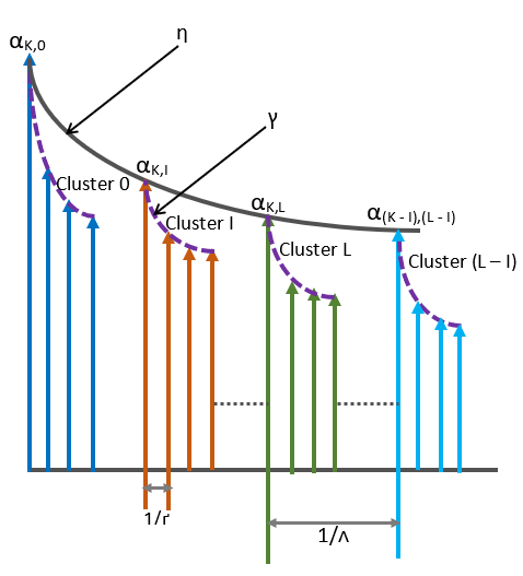
Fig 5.1: Saleh Valenzuela Channel Model distinguishing the cluster arrivals from the ray arrivals

5.2. Saleh Valenzuala Channel Model

Here in figure 5.1, it is shown Saleh Valenzuela model is basically based on amplitude and time delays of clusters and it is due to multi-paths between Tx & Rx. In figure the kth multi-path is forming many clusters like, cluster 0, cluster 1, etc., and each cluster contains rays.

Clusters are reaching at receiver at an average decay rate and similarly, rays or MPCs in each clusters are also forming in an average decay rate. The arrival rate of clusters and MPCs within each cluster is assumed to be governed by poisson distribution process (Meijerink, 2014).

Here, symbol ‘Λ’ representing the rate of clusters in unit time and ‘Γ’ represents the ray arrival rate in unit time.

When using the clustered channel model, the channel matrix H is supposed to be the sum of the contributions in the propagated multi-paths. As a result, channel matrix H can be expressed as
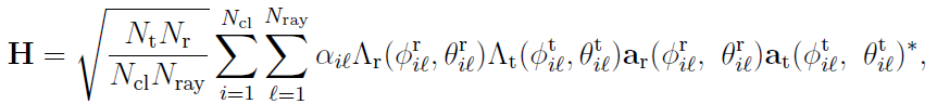
 30

…………(5.1)

(El Ayach, 2014)

Where,Ʌt (ϕtil θtil)= Gain of antenna elements at corresponding departure angles at tx

Ʌr (ϕril θril)= antenna element gain at the corresponding angles of arrival at rx

ar(ϕril θril)=normalized response vectors of antenna arrays at receiver with azimuth (elevation) angle of ϕril ( θril) and ϕtil ( θtil) respectively

ar(ϕril θril)=normalized response vectors of antenna arrays at receiver with azimuth (elevation) angle of ϕril ( θril) and ϕtil ( θtil) respectively

5.3. Different types of antenna arrays and their array response

The array response vectors for uniform linear arrays (ULA) with elements, N are represented as
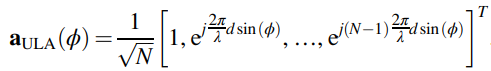
……….(5.2)

Similarly, for Uniform Planer arrays (UPA), the array response vectors can be represented as,

………..(5.3)

(Appendix A)

Where 0 ≤ x ≤ W1 -1 and 0 ≤ y ≤ W2 -1

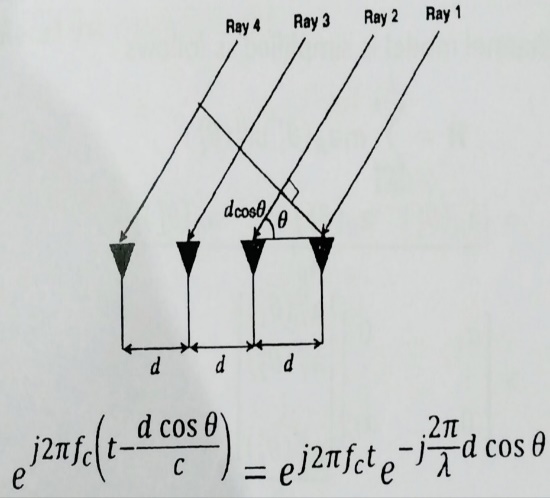
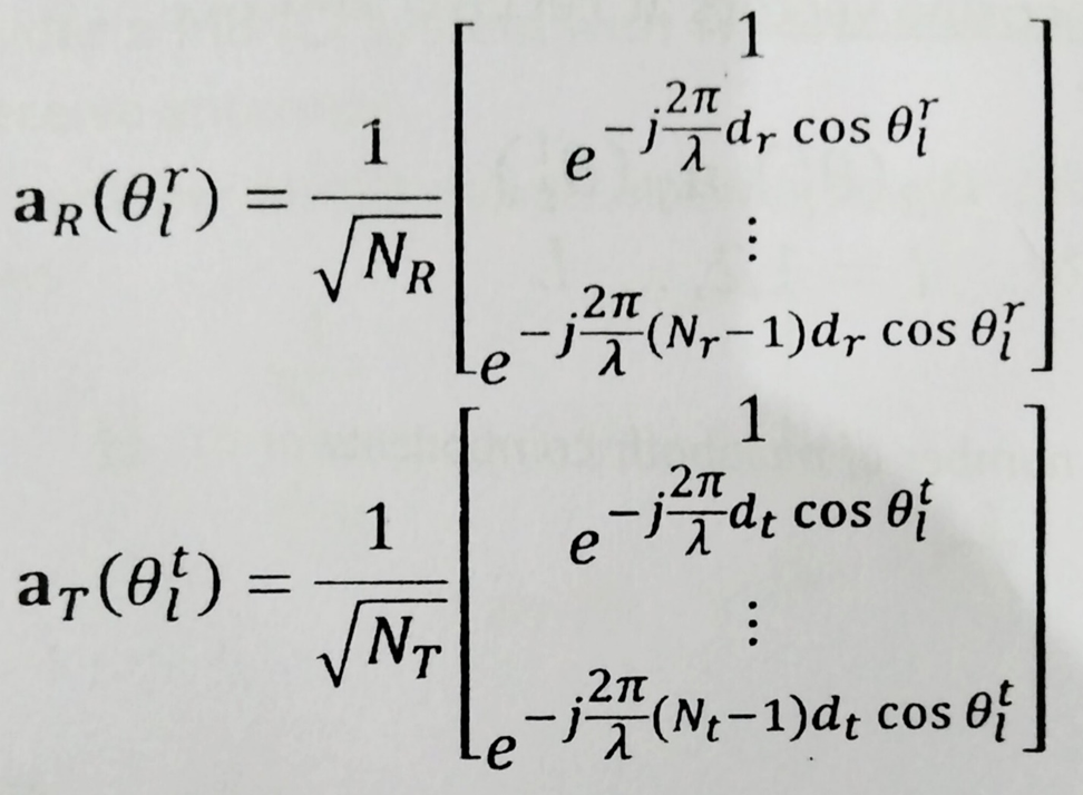
Fig 5.2: Directional cosine vectors at each antenna element (Appendix A)

In figure 5.2, it is illustrated that when transmitted signal reaches at receiver it creates different path lengths at different antenna element. Here in figure the second ray creates path-length difference of dcosθ with the first element. As there will be phase difference for same angle of departure (AOD) rays transmitted from Tx side. The corresponding calculation of phase difference is shown in figure.


People are good at skipping over material they already know!

View Related Topics to


Contact Us

Name

Email *

Message *

Popular Posts

Theoretical BER vs SNR for binary ASK, FSK, and PSK with MATLAB Code + Simulator

📘 Overview & Theory 🧮 MATLAB Codes 📚 Further Reading Bit Error Rate (BER) Equations BER formulas for ASK, FSK, and PSK modulation schemes. ASK BER = 0.5 × erfc(0.5 × √SNR) FSK BER = 0.5 × erfc(√(SNR / 2)) PSK BER = 0.5 × erfc(√SNR) Theoretical BER vs SNR for Amplitude Shift Keying (ASK) The theoretical Bit Error Rate (BER) for binary ASK depends on how binary bits are mapped to signal amplitudes. For typical cases: If bits are mapped to 1 and -1, the BER is: BER = Q(√(2 × SNR)) If bits are mapped to 0 and 1, the BER becomes: BER = Q(√(SNR / 2)) Where: Q(x) is the Q-function: Q(x) = 0.5 × erfc(x / √2) SNR : Signal-to-Noise Ratio N₀ : Noise Power Spectral Density Understanding the Q-F...

Simulation of ASK, FSK, and PSK using MATLAB Simulink (with Online Simulator)

📘 Overview 🧮 How to use MATLAB Simulink 🧮 Simulation of ASK using MATLAB Simulink 🧮 Simulation of FSK using MATLAB Simulink 🧮 Simulation of PSK using MATLAB Simulink 🧮 Simulator for ASK, FSK, and PSK 🧮 Digital Signal Processing Simulator 📚 Further Reading ASK, FSK & PSK HomePage MATLAB Simulation Simulation of Amplitude Shift Keying (ASK) using MATLAB Simulink In Simulink, we pick different components/elements from MATLAB Simulink Library. Then we connect the components and perform a particular operation. Result A sine wave source, a pulse generator, a product block, a mux, and a scope are shown in the diagram above. The pulse generator generates the '1' and '0' bit sequences. Sine wave sources produce a specific amplitude and frequency. The scope displays the modulated signal as well as the original bit sequence created by the pulse generator. Mux i...

BER vs SNR for M-ary QAM, M-ary PSK, QPSK, BPSK, ...(MATLAB Code + Simulator)

Bit Error Rate (BER) & SNR Guide Analyze communication system performance with our interactive simulators and MATLAB tools. 📘 Theory 🧮 Simulators 💻 MATLAB Code 📚 Resources BER Definition SNR Formula BER Calculator MATLAB Comparison 📂 Explore M-ary QAM, PSK, and QPSK Topics ▼ 🧮 Constellation Simulator: M-ary QAM 🧮 Constellation Simulator: M-ary PSK 🧮 BER calculation for ASK, FSK, and PSK 🧮 Approaches to BER vs SNR What is Bit Error Rate (BER)? The BER indicates how many corrupted bits are received compared to the total number of bits sent. It is the primary figure of merit for a...

OFDM Waveform with MATLAB Code

  In OFDM (Orthogonal Frequency Division Multiplexing) , we transmit multiple orthogonal subcarriers simultaneously. Since the subcarriers are orthogonal , they do not interfere with each other, which is one of the main advantages of OFDM. Practically, OFDM converts a wideband signal into multiple narrowband orthogonal subcarriers. For typical wireless communication, if the signal bandwidth (or symbol duration) exceeds the coherence bandwidth of the channel, the signal experiences frequency-selective fading . Fading distorts the signal, making it difficult to recover the original information. By using OFDM, we transmit the same wideband signal across multiple orthogonal narrowband subcarriers, reducing the effect of fading. For example, if we want to transmit a signal of bandwidth 1024 kHz , we can divide it into N = 8 subcarriers . Each subcarrier is then spaced by: Δf = Total Bandwidth N = 1024 8 kHz...

MATLAB Code for Constellation Diagram of QAM configurations such as 4, 8, 16, 32, 64, 128, and 256-QAM

📘 Overview of QAM 🧮 4-QAM MATLAB 🧮 16-QAM MATLAB 🚀 Online Simulator 📂 Other Topics on Constellation Diagrams... ▼ 🧮 MATLAB Code for 4-QAM 🧮 MATLAB Code for 16-QAM 🧮 MATLAB Code for m-ary QAM 🧮 Simulator for m-ary PSK 🧮 Simulator for m-ary QAM 🧮 Overview of Energy per Bit (Eb / N0) 🧮 Simulator for ASK, FSK, and PSK Overview of QAM One of the best-performing modulation techniques is QAM [↗] . Here, we modulate the symbols by varying the carrier signal's amplitude and phase in response to the variation in the message signal (or voltage variation). So, we may say that QAM is a combination of phase and amplitude modulation. Additionally, it performs better than ASK or PSK [↗] . In fact, any constellation for any type of modulatio...

Power Spectral Density Calculation Using FFT in MATLAB

📘 📘 Overview 🧮 🧮 Steps to calculate 💻 🧮 MATLAB Codes 📚 📚 Further Reading Power spectral density (PSD) tells us how the power of a signal is distributed across different frequency components, whereas Fourier Magnitude gives you the amplitude (or strength) of each frequency component in the signal. Steps to calculate the PSD of a signal Firstly, calculate the fast Fourier transform (FFT) of a signal. Then, calculate the Fourier magnitude (absolute value) of the signal. Square the Fourier magnitude to get the power spectrum. To calculate the Power Spectral Density (PSD), divide the squared magnitude by the product of the sampling frequency (fs) and the total number of samples (N). Formula: PSD = |FFT|^2 / (fs * N) Sampling frequency (fs): The rate at which the continuous-time signal is sampled (in Hz). ...

Online Simulator for ASK, FSK, and PSK

Try our new Digital Signal Processing Simulator!   •   Interactive ASK, FSK, and BPSK tools updated for 2025. Start Now Interactive Modulation Simulators Visualize binary modulation techniques (ASK, FSK, BPSK) in real-time with adjustable carrier and sampling parameters. 📡 ASK Simulator 📶 FSK Simulator 🎚️ BPSK Simulator 📚 More Topics ASK Modulator FSK Modulator BPSK Modulator More Topics Simulator for Binary ASK Modulation Digital Message Bits Carrier Freq (Hz) Sampling Rate (...

FastAPI Static Files – Overview

FastAPI Static Files Often, a web application needs to include resources that do not change, even when dynamic data is rendered. These resources are called static assets . Examples of static files include: Images ( .png , .jpg ) JavaScript files ( .js ) Stylesheets ( .css ) Installing Required Library To handle static files in FastAPI, you need the aiofiles library. pip install aiofiles Mounting Static Files FastAPI uses the StaticFiles class to serve static content. You mount a folder (usually named static ) so that all files inside it can be accessed via a URL. from fastapi import FastAPI from fastapi.staticfiles import StaticFiles app = FastAPI() app.mount("/static", StaticFiles(directory="static"), name="static") Example 1: Using an Image Place an image file (for example, fa-logo.png ) inside the static folder. main.py from fastapi import FastAPI, Request from fastapi.responses import HTMLRespon...