Millimeter wave 5G

Millimeter wave 5G

Introduction

In fifth-generation (5G) mobile networks, millimetre wave (mm Wave) communication is one of the most favourable technologies. It has access to a huge amount of available spectrum. In spite of the theoretical potential of high speed data, the use of mm wave in mobile networks experience number of major technical challenges, including significant path loss, narrow beam width, high penetration loss, etc. Cisco IBSG predicted that by 2020, there will be 50 billion Internet- connected devices (Ahmed, 2018). In the next ten years, mobile data traffic will increase by a factor of 1000. Mm-wave bands with massive MIMO systems will help meet these needs because massive MIMO allows to produce a narrow beam with high spectrum efficiency to the user. Narrow beam and spatial multiplexing in MIMO is responsible for high data rates.

1.1. Fundamental Characteristics of millimetre wave:

Millimetre wave wavelength ranges from 1 mm to 10 mm. It has several basic features, including large bandwidth, severe path loss, narrow beam width, high penetration loss, etc.

1.1.1. Large amount of bandwidth:

Now a days, for many mobile networks, total operating bandwidth spectrum is less than 780 MHz, including 4G, which is not enough to meet the high data rate requirements from different devices. One of the major advantages of mm wave communication compared to conventional communication with microwaves is the significantly larger bandwidth spectrum. Although some unfavorable bands, e.g, 57-64 GHz are easily absorbed by oxygen and 164-200 GHz bands by water vapour. For mm wave communications, the appropriate bandwidth is still greater than 150 GHz (Lin, 2019).

1.1.2. Propagation Loss:

In general, propagation loss can be interpreted as both path loss and penetration loss. For line-of-sight (LOS) conditions, free space path loss is proportional to the square of operating carrier frequency, according to the Friis transmission formula. The propagation loss in the mm Wave band is much higher than in the microwave band because the frequency range is 30 GHz to 300 GHz. A high-gain directional antenna, on the other hand, can be used to compensate (Lin, 2019).

Even though one of the disadvantages of the mm wave is severe path loss, the good side is that the combination of mm Wave with device-to-device (D2D) communication has relatively low multi-user interference because of the high pathloss and use of directional antennas. This combination can support huge amounts of simultaneous D2D links, such that the network capacity can be further improved. Additionally, a higher security against eavesdropping and jamming can be obtained. In non-line-of-sight scenarios (NLOS), the penetration loss is usually higher at higher frequencies. As a consequence, covering indoor spaces with mm Wave nodes with outdoor nodes is a difficult job. Signals must pass through the building walls for indoor users connected to an outdoor base station (BS). The data rate, spectral and energy efficiency of this propagation all suffer significantly because of penetration losses. The higher the carrier frequency, the worse the situation (Lin, 2019).

Received signal power in atmospheric environment can be defined as

P_r = P_t + G_t + G_r + 20log₁₀(λ/4πd) + atmospheric pathloss………(1.1)

λ = wavelength of carrier frequency

d = distance between Tx & Rx

G_t, G_r = transmitter & receiver antenna gain, respectively

20log₁₀(λ/4πd) = free space pathloss at first propagation reference distance d

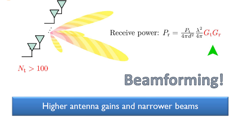
Fig 1.1: Illustration of beamforming using massive MIMO antenna

Because of small wavelength, it suffers from huge path loss. Massive MIMO beamforming is required to combat high path loss as shorter wavelength allows Compact antenna arrays in a small region. More antenna elements in a small region gives more beamforming gain. In figure 1.1, it is shown closely spaced antenna elements are forming beam in a particular direction. Usually antenna elements are spaced in half-wavelength interval to avoid unwanted sidelobes and to focus stronger signal in a particular direction.

1.1.3. Short Wavelength:

The MM wave signal has a much shorter wavelength than the microwave signal, which is in the order of millimeters. Therefore, it is considered essential for mm wave communication, since short wavelengths at mm wave frequencies are suitable to pack a lot of half-wavelength spaced antenna elements into a compact space,

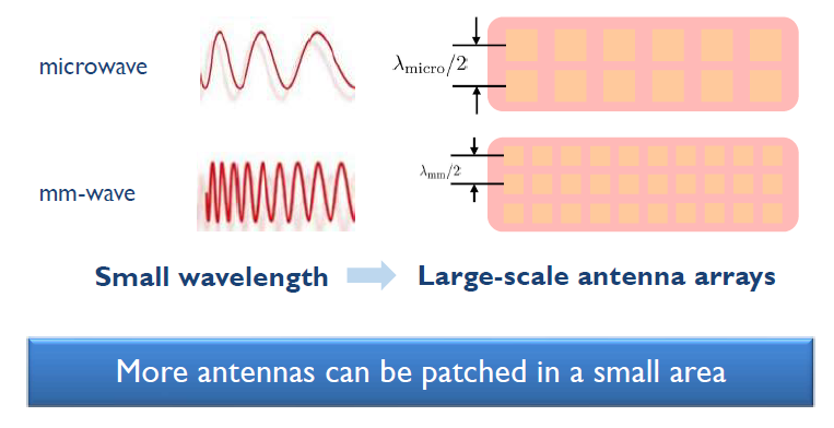
Fig 1.2: Comparison of number of antenna elements spaced in same area to achieve higher antenna correlation gain with more antenna element spaced in half-wavelength interval and to reduce multiple sidelobes

Here in above figure 1.2, we can see, in case of millimetre wave band communication, we can place more antenna elements in half-wavelength interval in a compact are rather than microwave band communication. The more antenna element, more narrower beam and that leads to higher beamforming gain. A massive MIMO system equipped with large antenna arrays has enough capability to improve spectral efficiency by transmitting same signal from many antenna elements. Moreover, spatial, time, and frequency diversity is also possible.

1.2. Millimetre wave vehicular communication:

Future self-driving cars would need up to 1 TB of data per hour of driving, with data speeds above 750 Mbit/s. This highlights the limitations of modern wireless technologies for automotive data sharing and justifies the use of mm wave spectrum for greater data availability and reduced latency due to the much wider bandwidth allocations. Moreover, as a supporter of the concept of fully connected vehicles, the NLOS transmission is a major issue for mm-wave communication (Antonescu, 2017). 5G communication is growing interest in the automotive industry due to its low latency and larger bandwidth spectrum. Vehicular communication operates on highly dynamic condition where communication nodes are not like common cellular networks because, here channel is time-varying and network topology also varies fast due to high mobility. If mobility is high, then channel impulse response varies fast, that dramatically reduces the coherence time in compare to common cellular networks. Coherence time is denoted by in wireless communication CIRs experiences almost same attenuation in a particular time interval during data transmission. As dynamic channel impulse response is changing very fast, so obtaining high beamforming gain also becomes challenging. Hence, we need to estimate the time-varying channel in extremely short time duration (Garcia, 2016).

1.3. Millimetre wave 5G indoor communication:

In terms of indoor networks, 5G means innovative user features, new organisational productivity opportunities by IoT, factory automation, and new networking services. 5G will implement completely modern architectures to enable Massive IoT and Critical Realtime IoT applications, in addition to developments in multi-Gbps mobile broadband. Wireless communication is also becoming popular in industrial operation day by day due to its low reliable latency. It is needed to control appliances i.e, automated vehicles, machine to machine communication in factories, etc. compare to wired communication, and wireless communication is cost efficient. UWB and millimetre wave bands are suitable for enabling high data rate indoor communication. UWB band can detect the position of devices in accuracy range of 5-10 centimetre and millimetre wave in millimetre range (Frenzel, 2007). UWB and millimetre wave can measure the angle of arrival and angle of departure by calculating phase difference between antenna elements. Saleh Valenzuala model is widely adopted for indoor communication which is based on amplitude and time delay model to form clusters. Because of its advantages in industry, wireless networking is increasingly growing to new heights (Traβl, 2019). Most of the channel models are characterized by empirical, statistics, or stochastic model. An empirical channel model is developed for a particular application. So, deterministic channel models e.g, ray tracing model is becoming popular which is based on fresnel coefficient, farmat’s law and electromagnetic propagation theory (Sidhu, 2012).