Mm-Wave Channel pathloss Model

Mm-Wave Channel pathloss Model

4.1. Introduction

The propagation loss of millimeter wave band is much higher due to its higher operating frequency. Due to higher frequency it has a stronger reflectivity property when it interacts with buildings, glasses, metals, etc and it is easily absorbed by atmospheric gases, rain, etc, compare to lower frequency bands. On the other hand, the penetration loss, especially for non-line of sight (NLOS) condition is larger in higher frequencies. It becomes difficult to cover the indoor spaces while base station is deployed in outside because the building wall or any obstacle leads very high penetration loss. It significantly degrades the signal power, and spectral efficiency. 5G networks to fulfill high data requirements by applying mm-wave wireless backhaul, small cells, in band full duplex and device to device (D2D) communication. The high pathloss and the narrower beamwidth in mm-wave communication, is positive for device to device communication with less interference (Lin, 2019).

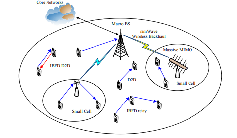
Fig 4.1. Illustration of promising technologies in 5G networks

4.2. Large scale parameters (LSPs)

Path loss, shadowing loss have major effects that impact the power received in a receiver thru radio channel. These two are critical in evaluating the characteristics of radio channel’s large-scale parameters. Increasing the distance between Tx and Rx degrades the signal strength, resulting in path loss. The path loss exponent ‘n' demonstrates how fast pathloss grows in different environments (Antonescu, 2017). The shadowing loss due to the blocking and absorption of propagated signal by barriers and scattering, respectively, is considered as large-scale pathloss.

4.3. Small scale parameters (SSPs)

Path loss due to fading is characterized as small scale pathloss. Multi-path components and doppler spread are responsible for fading. Small scale parameters are evolved in angle of arrival (AOA) & angle of departure (AOD). So, it is also involved in cluster birth & death. Cluster is defined as when multi-paths comes from different directions and they are close in time (Ju, 2018).

4.4. Pathloss:

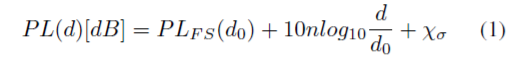
In case of millimetre wave communication channel propagation model is realized by close in pathloss. Close-in pathloss model is a great approach that covers wide distances with great precision. The goal is to produce model of large-scale channel propagation. Log-normal distribution is usually used to demonstrate the channel model where the distribution has standard deviation and zero mean value (Antonescu, 2017).

……………(4.1)

(Antonescu, 2017)

Where, PL(d₀) is the free-space loss at reference distance d₀

n = pathloss exponent

χ_σ = shadowing factor with zero-mean Gaussian random variable with a standard deviation σ in dB. Standard deviation indicates how much the instantaneous pathloss varied from average value.

PL_FS(d₀) indicates pathloss at 1^st one meter propagation of mm wave.

Pathloss depends on the operating frequency and distance between Tx and Rx and pathloss exponent ‘n’ for a particular environment (Ju, 2019). If there is no line of sight between our TX and RX, the radio waves come to the receiver from multiple directions, with differing transmission delays due to reflection and scattering. The multi-path components (MPCs) including multipath elements, randomly distributed amplitude, phase and angle-arrival (AOAs) combine in receiver to distort the received signal. In addition to multi-paths, the Doppler spread caused by the mobility and speed of Tx and Rx has an affect on the small-scale propagation channel model. Small-scale effects are characterised as rapid changes in obtained signal intensity over a short path or time interval because of Doppler shifts, and as signal arrives from Tx to Rx thru multi-paths, it causes time dispersion (different delay in different MPCs) in received signal that leads to inter-symbol interference. The type of fading is defined by the relationship between signal parameters (bandwidth, symbol period) and channel parameters (Doppler spread/Coherence time or bandwidth) in a radio channel. So, multi-paths produce different types of fading because multi-path delay spread and doppler spread (Antonescu, 2017).

4.5. Spatial Consistency Procedure:

Spatial consistency is demonstrated by consistent and practical channel impulse response along the UT pathway in a local environment. Spatial consistency produces time-variant small-scale parameters such as angle of arrival (AOA) and departure (AOD), control, delay, and phase per MPC, as well as spatially associated large-scale parameters such as Shadow fading (SF), LOS, and NLOS conditions. The "local region" is defined by the correlation distances of the large scale parameters (LSPs), which defines the length of a channel segment (typically 10–15 m). The channels in a channel section are assumed to be strongly correlated and modified using the spatial consistency method. Depending on the RSSI of the receiver signal. A channel section can be divided into various regions. Here I have shown Spatial consistency and rms delay spread by MS varying velocity 8 m/sec (approx. 29km/h), 16 m/sec (approx. 58km/h), and 30 m/sec (approx. 108km/h) (Ju, 2019).