Orthogonal Frequency Division Multiplexing
When a signal with high bandwidth traverses through a medium, it tends to disperse more compared to a signal with lower bandwidth.
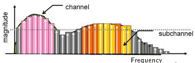
A high-bandwidth signal comprises a wide range of frequency components. Each frequency component may interact differently with the transmission medium due to factors such as attenuation, dispersion, and distortion. OFDM combats the high-bandwidth frequency selective channel by dividing the original signal into multiple orthogonal multiplexed narrowband signals. In this way it, overcomes the inter-symbol interferences (ISI) issue.
Block Diagram

‘k’ indicates kth position in a input symbol
N is the number of subcarriers
Example: (OFDM using QPSK)
1.
Input Parameters:
N Number of Input bits: 128
Number of subcarriers (FFT length): 64
Cyclic prefix length (CP): 8
Step-by-Step Process:
QPSK Mapping:
Each QPSK symbol represents 2 bits.
‘With 128 bits, the number of QPSK symbols generated will be 64 symbols.
2. OFDM Symbol Construction:
The 64 QPSK symbols exactly fit into 64 subcarriers, meaning we form one OFDM
symbol
3. IFFT Operation:
Each OFDM symbol (composed of 64 QPSK symbols) is transformed from the
frequency domain to the time domain using a 64-point IFFT.
The output of the IFFT is 64 complex time-domain samples per OFDM symbol.
4. Adding Cyclic Prefix:
A cyclic prefix of length 8 is appended to each 64-sample time-domain OFDM
symbol.
Therefore, each OFDM symbol with the cyclic prefix becomes 64 + 8 = 72 samples
long.
5. Total Length of OFDM Modulated Signal:
Since we have only one OFDM symbol in this example, the total length of the OFDM
modulated signal is 72 samples.
MATLAB Code for a simple OFDM system
% The code is written by SalimWireless.Com
clc;
clear all;
close all;
% Generate random bits
numBits = 100;
bits = randi([0, 1], 1, numBits);
% Define parameters
numSubcarriers = 4; % Number of subcarriers
numPilotSymbols = 3; % Number of pilot symbols
cpLength = ceil(numBits / 4); % Length of cyclic prefix (one-fourth of the data length)
% Add cyclic prefix
dataWithCP = [bits(end - cpLength + 1:end), bits];
% Insert pilot symbols
pilotSymbols = ones(1, numPilotSymbols); % Example pilot symbols (could be any pattern)
dataWithPilots = [pilotSymbols, dataWithCP];
% Perform OFDM modulation (IFFT)
dataMatrix = reshape(dataWithPilots, numSubcarriers, []);
ofdmSignal = ifft(dataMatrix, numSubcarriers);
ofdmSignal1 = reshape(ofdmSignal, 1, []);
% Display the generated data
disp("Original Bits:");
disp(bits);
disp("Data with Cyclic Prefix and Pilots:");
disp(dataWithPilots);
disp("OFDM Signal:");
disp(ofdmSignal1);
%%%%%%%%%%%%%%%%%%%%%%%%%%% Demodulation %%%%%%%%%%%%%%%%%%%%%%%%%%%%%%%%%%
% Perform FFT on the received signal
%ofdmSignal = awgn(ofdmSignal, 1000);
ofdmSignal = reshape(ofdmSignal1, numSubcarriers, []);
rxSignal = fft(ofdmSignal, numSubcarriers);
%rxSignal = [rxSignal(1,:) rxSignal(2,:) rxSignal(3,:) rxSignal(4,:)];
% Remove cyclic prefix
rxSignalNoCP = rxSignal(cpLength + 1:end);
% Extract data symbols and discard pilot symbols
dataSymbols = rxSignalNoCP(numPilotSymbols + 1:end);
% Demodulate the symbols using thresholding
threshold = 0;
demodulatedBits = (real(dataSymbols) > threshold);
figure(1)
stem(bits);
legend("Original Information Bits")
figure(2)
% Plot real part
hReal = stem(real(ofdmSignal1), 'r', 'DisplayName', 'Real Part'); % 'r' for red color
hold on;
% Plot imaginary part
hImag = stem(imag(ofdmSignal1), 'b', 'DisplayName', 'Imaginary Part'); % 'b' for blue color
% Customizing the plots
set(hReal, 'Marker', 'o', 'LineWidth', 1.5); % Real part marker and line style
set(hImag, 'Marker', 'x', 'LineWidth', 1.5); % Imaginary part marker and line style
% Add grid and other plot customizations
grid on;
title('Real and Imaginary Parts of OFDM Signal');
xlabel('Index');
ylabel('Amplitude');
legend;
hold off;
figure(3)
stem(demodulatedBits);
legend("Received Bits")
Output


OFDM is a scheme of multicarrier modulation. It's utilized to make greater use of the spectrum. Multiple carriers are used to modulate the message signal in this case. According to Nyquist's sampling theorem, to perfectly reconstruct a baseband signal with a maximum frequency component of fmax, we must sample the signal at a rate of at least 2*fmax. For a passband signal, the sampling rate depends on its bandwidth. The text also mentions a relationship between bandwidth B and 2*fmax, which needs clarification. Generally, the bandwidth B of a baseband signal is fmax. For a passband signal, it's typically the difference between the upper and lower frequency limits.
Multi-path components, or MPCs, are seen while transmitting a signal in a wireless environment. MPCs are numerous copies of the same transmitted signal that arrive at the receiver with time delay or dispersion. If we send the second symbol immediately after the first, the second symbol will interact with the first symbol's time delayed MPCs. Excess delay spread refers to the time gap between the first and last MPCs. However, for measuring the time dispersion of multi path components, or MPCs, RMS delay spread is the most appropriate term. The RMS delay spread is the power delay spread's second central momentum, taking into account the relevant power weightage associated with MPCs. You've probably noticed signal power delay spread owing to multi-path in a wireless context.
Assume that the total bandwidth available is B. The symbol duration of a single carrier system is approximately 1/B. Signals at higher frequencies are subjected to additional reflection and refraction, creating more multipath and causing the signal to reach the receiver via several reflections and refractions. RMS delay spread (say, Td) can be substantially more than the symbol time length (say, Ts) or Td>>Ts in such circumstances (especially for very high frequency channels). When the RMS delay spread is greater than the symbol time length, the symbol interacts with the MPCs of other symbols. This is technically termed Inter-symbol interference, or ISI.
We divide the entire available bandwidth B into N number of sub-bands to mitigate inter-symbol interference. The bandwidth of each sub-band will be B/N. The symbol duration, Ts, for each sub-band will be 1/(B/N). This symbol duration, Ts, will be significantly larger than 1/B. Common values for N are 256, 512, and so on. In the OFDM approach, we often utilize N-point FFT for multi-carrier modulation, or MCM.
Let me explain using a mathematical example: the RMS delay spread for an outdoor communication channel is typically 2 to 3 microseconds. If we use single carrier transmission with a transmission bandwidth of 10 MHz, the symbol time duration is Ts = 1/B = 1/(10 * 10^6) = 0.1 microsecond. Since Td (=2 to 3 microsecond) is greater than Ts (=0.1 microsecond), Inter-symbol interference, or ISI, is the result of this.
If we divide the broadband bandwidth, B, into N sub-bands, the bandwidth of each sub-band becomes B/N, significantly increasing the symbol time duration, Ts. We normally aim for symbol duration periods to be significantly longer than the RMS delay spread (e.g., 10 times longer) for seamless communication. This principle helps in avoiding ISI.
Diagram:
Here's an illustrative diagram for conventional single carrier transmission:

In the diagram above, a traditional single carrier communication system is depicted. B is the total bandwidth. If B = 10 MHz, Ts = 1/(10 MHz) = 0.1 microsecond symbol duration. RMS delay spread, Td = 2 - 3 microsecond. As a result, the RMS delay spread is greater than the symbol time. This leads to issues where the desired signal is not cleanly recoverable. To address this, in the next diagram, we demonstrate how the entire bandwidth B is divided into N (say, 1000) portions.
Here's a diagram illustrating multicarrier transmission in OFDM:

Each sub-band's bandwidth is now B/N. Multicarrier modulation is used to modulate the sub-band message signal. If B = 10 MHz and N = 1000, then each sub-band has a bandwidth of (10 MHz)/1000 = 10 KHz. Each sub-band's symbol time, Ts, is now equal to 1/(10KHz) = 100 microsecond. The symbol time (100 microseconds) is significantly higher than the critical RMS delay spread (2-3 microseconds) in this case. Theoretically, that is enough to remove ISI.
Filter Bank Multi-Carrier (FBMC)
'FBMC' is the abbreviation for 'Filter Bank Multi-Carrier.' In an OFDM system, we use Inverse Fast Fourier Transform (IFFT) at the transmitter side and Fast Fourier Transform (FFT) at the receiver side to process the subcarriers. For OFDM, we use the term Tsym, which stands for symbol duration time. As we know, it's a multi-carrier modulation system in which we send a single high data rate signal broken into multiple low data rate signals in parallel. To cancel inter-symbol interference (ISI) in a communication system caused by fading, we divide the entire bandwidth B into N sub-bands.
One of the main drawbacks of OFDM systems is that the subcarrier filters of the IFFT/FFT filter banks have poor spectral containment. As a result, there is significant interference from other users' transmissions or adjacent subcarriers.
Additionally, when transmitting a symbol in OFDM, we must not only use the Tsym time period, but also add a cyclic prefix. This phenomenon impacts bandwidth efficiency.
Another explanation is that when we send a signal over a multicarrier system, the spectral response of each carrier signal often behaves like a sinc function. As a result, every subcarrier can interfere with the subcarriers before and after it (out-of-band emissions).
FBMC resolves these concerns with the OFDM system. To differentiate the subcarriers, FBMC utilizes a digital filter bank with better spectral localization. We also typically don't require the cyclic prefix in this case, improving bandwidth efficiency. Digital filters are designed to be sharp in nature, significantly reducing interference between other subcarriers.
# OFDM delay spread channel to parallel fading channel conversion
Q & A and Summary
1. What is the main advantage of using Orthogonal Frequency Division Multiplexing (OFDM) in wireless communication?
Answer: The main advantage of OFDM is its ability to overcome inter-symbol interference (ISI) caused by frequency-selective fading in high-bandwidth channels. By dividing the original signal into multiple narrowband signals, OFDM ensures that each subcarrier experiences less distortion, making it more robust against channel impairments like attenuation, dispersion, and distortion. Additionally, the orthogonality between subcarriers ensures minimal interference, reducing ISI and improving overall system performance.
2. How does OFDM transform a frequency-selective channel into multiple frequency-flat channels?
Answer: OFDM works by dividing the original high-bandwidth signal into multiple narrowband subcarriers. Each subcarrier operates at a lower data rate, making it less susceptible to frequency-selective fading. This approach transforms a frequency-selective channel into several parallel, frequency-flat channels. The orthogonality between subcarriers ensures minimal interference and allows data to be transmitted across them efficiently.
3. What role does the Inverse Fast Fourier Transform (IFFT) play in OFDM?
Answer: The Inverse Fast Fourier Transform (IFFT) is crucial in OFDM. It is used to convert the frequency-domain data symbols into time-domain signals. After the data is divided into subcarriers, the IFFT is applied to combine them into a single time-domain signal that can be transmitted. This operation ensures that the subcarriers remain orthogonal, preventing interference between them during transmission. Mathematically, the IFFT is represented as:
$$ y(t) = \sum_{k=0}^{M-1} X_k e^{j2\pi k t / T} $$
Where $X_k$ are the frequency-domain symbols, and $y(t)$ is the resulting time-domain signal.
4. What is the function of the cyclic prefix in an OFDM system, and why is it necessary?
Answer: The cyclic prefix is a copy of the last part of each OFDM symbol added at the beginning of the symbol. Its purpose is to mitigate the effects of multipath delay spread in the wireless channel. Without it, multipath propagation would lead to inter-symbol interference (ISI) due to overlapping symbols. The cyclic prefix provides a guard interval that prevents overlap between successive symbols, thus helping maintain the orthogonality between subcarriers. The cyclic prefix $T_{cp}$ length is typically chosen to be longer than the maximum delay spread of the channel.
5. How does high Doppler shift affect the performance of an OFDM system?
Answer: High Doppler shift leads to a loss of orthogonality between the subcarriers in an OFDM system. When the relative speed between the transmitter and receiver is high, the frequency of the received signals may shift, causing inter-carrier interference (ICI). This degradation results in poor bit error performance, particularly in environments where the channel characteristics change rapidly, leading to persistent errors or "error floors." Mathematically, the Doppler shift $\Delta f$ is related to the relative velocity $v$ by the equation:
$$ \Delta f = f_0 \cdot \frac{v}{c} $$
Where $f_0$ is the frequency of the subcarrier, $v$ is the relative velocity between the transmitter and receiver, and $c$ is the speed of light.
6. What is the concept of "orthogonality" in the context of OFDM, and why is it crucial for the system's performance?
Answer: Orthogonality in OFDM refers to the property that ensures that the subcarriers do not interfere with each other despite overlapping in frequency. The subcarriers are chosen such that their frequency components are mathematically orthogonal to each other, ensuring zero cross-talk between them. This prevents inter-carrier interference (ICI) and allows multiple signals to be transmitted simultaneously on the same channel, thus improving spectral efficiency. The orthogonality condition is maintained by ensuring the following condition holds for all pairs of subcarriers:
$$ \int_0^T e^{j 2 \pi f_{k_1} t} e^{-j 2 \pi f_{k_2} t} dt = 0 $$
Where $f_{k_1}$ and $f_{k_2}$ are the frequencies of two different subcarriers, and $T$ is the symbol period.
7. What are the main steps involved in the OFDM transmitter process?
Answer: The main steps involved in the OFDM transmitter process are as follows:
- Data Encoding: Convert the input data stream into symbols suitable for transmission (e.g., using QAM or PSK modulation).
- Serial-to-Parallel Conversion: Group the symbols into blocks and convert them into parallel data streams, one for each subcarrier.
- Inverse Fast Fourier Transform (IFFT): Apply the IFFT algorithm to convert the time-domain parallel data streams into frequency-domain OFDM symbols.
- Cyclic Prefix Addition: Add a cyclic prefix to each OFDM symbol to handle multipath delay spread.
- Digital-to-Analog Conversion: Convert the time-domain OFDM symbols into analog signals.
- Upconversion and Transmission: Upconvert the analog OFDM signal to the desired carrier frequency and transmit it.
8. What happens at the receiver side of an OFDM system, and how does the receiver handle channel impairments?
Answer: At the receiver side, the following steps occur:
- Signal Reception: Receive the transmitted OFDM signal after it has traveled through the wireless channel.
- Downconversion: Downconvert the received signal to baseband or an intermediate frequency.
- Analog-to-Digital Conversion: Convert the analog signal into a digital form suitable for processing.
- Cyclic Prefix Removal: Remove the cyclic prefix from each OFDM symbol.
- Fast Fourier Transform (FFT): Apply FFT to convert the time-domain symbols back into the frequency domain.
- Parallel-to-Serial Conversion: Convert the frequency-domain symbols back into a serial data stream.
- Data Demodulation: Demodulate the received symbols to recover the original data stream.
- Channel Equalization: Apply equalization techniques to mitigate frequency-selective fading and other channel impairments.
- Data Decoding: Decode the received symbols to retrieve the original data stream.
9. Explain the concept of "frequency-selective fading" and its impact on OFDM systems.
Answer: Frequency-selective fading occurs when different frequency components of a signal experience different levels of attenuation due to the channel’s characteristics, such as multipath propagation. OFDM combats this by dividing the signal into multiple narrowband subcarriers, each of which is less affected by the fading. This transforms a frequency-selective channel into several parallel, frequency-flat channels, which helps reduce distortion and improve the overall system's reliability.
10. How does OFDM improve spectral efficiency in wireless communication systems?
Answer: OFDM improves spectral efficiency by allowing the transmission of multiple data streams simultaneously on different subcarriers that are closely spaced in frequency. The orthogonal nature of the subcarriers ensures that the signals do not interfere with each other, thus maximizing the use of the available bandwidth. Additionally, the ability to adapt the modulation scheme for each subcarrier depending on the channel conditions further enhances spectral efficiency. The result is a more efficient use of the spectrum, which is especially beneficial in high-density communication environments.
Further Reading
